Adding a new variable to the Dictionary
new_variable_to_dict.RmdThis is a vignette to describe the process to add a new variable to the Dictionary of the package. This is necessary if we want to use a new variable in the OSEM Model. Here we initially discuss three cases: 1) the case of adding a Eurostat variable and 2) adding a new variable from the EDGAR emission dataset and lastly 3) to simply create a new identity based on existing variables.
tl,dr
This is an example how you add a new variable to the Dictionary:
# Add a new row to 'dict', which is an element of the osem package
dict %>%
  bind_rows(tibble(
    model_varname = "IndProd", # this is free to choose but must be unique
    full_name = "An index of Industrial Production",
    database  = "eurostat",
    variable_code = "PRD", # in this case use the bt_indicator information here
    dataset_id = "sts_inpr_q",
    var_col = "indic_bt", # here we specify what the column with the variables is called
    freq = "q", # for quarterly data, 'm' would be monthly
    geo = "AT",
    unit = "I15", # for index of 2015 = 100
    s_adj = "NSA", # not seasonally adjusted
    nace_r2 = "B-D")) -> new_dict

# now use the new_dict in run_model
Some general remarks about the Dictionary
The dictionary is the central store of information that is being used for us to “translate” difficult data codes into useful variable names - and it is also central for us to tell the OSEM Model what to download.
Let’s take a look at the dictionary:
dict %>% as_tibble %>% slice(1:10)
#> # A tibble: 10 × 33
#>    model_varname full_name variable_code database dataset_id var_col freq  geo
#>    <chr>         <chr>     <chr>         <chr>    <chr>      <chr>   <chr> <chr>
#>  1 Supply        Total Su… NA            NA       NA         NA      NA    NA
#>  2 Demand        Total De… NA            NA       NA         NA      NA    NA
#>  3 GDPOutput     GDP Outp… NA            NA       NA         NA      NA    NA
#>  4 GDPExpenditu… GDP Expe… NA            NA       NA         NA      NA    NA
#>  5 CO2Industry   Co2 Emis… NA            NA       NA         NA      NA    NA
#>  6 TOTS          Total Su… TOTS          NA       NA         NA      NA    NA
#>  7 DomDemand     Domestic… DomDemand     NA       NA         NA      NA    NA
#>  8 ATaxesA       Product … D21           eurostat nama_10_g… na_item a     DE
#>  9 ASubsidiesA   Product … D31           eurostat nama_10_g… na_item a     DE
#> 10 CO2Agricultu… CO2 Emis… CO2           eurostat env_ac_ai… airpol  a     DE
#> # ℹ 25 more variables: unit <chr>, s_adj <chr>, nace_r2 <chr>, cpa2_1 <chr>,
#> #   sector <chr>, direct <chr>, age <chr>, partner <chr>, finpos <chr>,
#> #   p_adj <chr>, meat <chr>, citizen <chr>, wstatus <chr>, tra_oper <chr>,
#> #   ipcc_sector <chr>, GEO <chr>, `Seasonal adjustment` <chr>,
#> #   `North American Industry Classification System (NAICS)` <chr>,
#> #   `North American Product Classification System (NAPCS)` <chr>, Prices <chr>,
#> #   `Type of fuel` <chr>, `Products and product groups` <chr>, …
A few words about the variables/columns in the dictionary: There are a few crucial columns that will nearly always be needed/useful. These are:
model_varname: Variable name in the model equations, must be unique.
full_name: Full name/description of the variable.
Currently full in use are also the columns:
database: Name of the database. Internally implemented are “eurostat” and “edgar.”
variable_code: Identifier of the variable if applicable, e.g., Eurostat variable code.
dataset_id: Identifier of the dataset where the variable is available, e.g., Eurostat dataset code or link to file on the web.
More varied is the use of:
var_col: Name of variable/column in the dataset.
freq: Frequency of the variable in the dataset. “m” for monthly, “q” for quarterly.
geo: ISO 3166-1 alpha-2 country code.
unit: Eurostat unit in which the variable is measured, e.g., to choose between different measurements for the same variable.
s_adj: Eurostat seasonal adjustment or not.
nace_r2: Eurostat identifier for NACE Rev. 2 classification.
ipcc_sector: EDGAR IPCC National Greenhouse Gas Inventories, see link. “TOTAL” is not an official IPCC code but is internally interpreted to use country totals.
cpa2_1: Eurostat identifier for Classification of Products by Activity (CPA).
siec: Standard International Energy Product Classification, e.g., for Eurostat.
Adding a variable from Eurostat
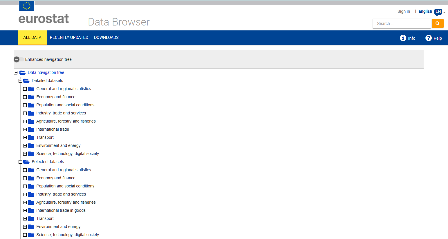
Firstly, head over to Eurostat to find out more about the variable you would like to add. There are a few data viewer options in Eurostat, but we recommend using the “Data Explorer” for this. Here is a good link to get started:
Eurostat Data Viewer Data Navigation Tree
Identifying the correct information needed
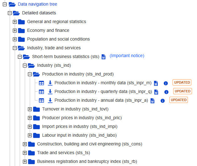
Now let’s assume that we want to add some form of Industrial
Production to the dataset (Link).
So we head back to the data tree and select the quarterly dataset for
Industrial Production (sts_inpr_q):
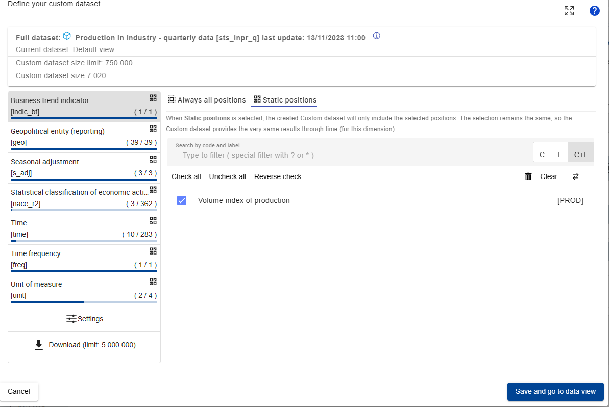
Now let’s take a closer look at the data features that are typically at the top of the screen:
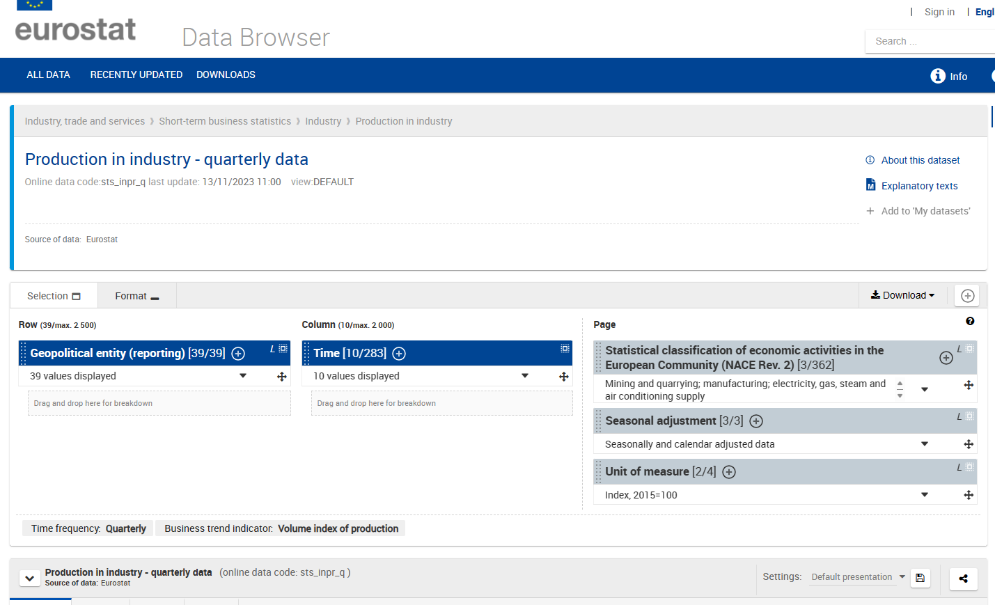
This already gives us something crucial: the dataset identifier, in
this case sts_inpr_q. This corresponds to the column
dataset_id in the Dictionary dict.
To find out even more about all the detailed features of the dataset,
we click on the big encircled + that are e.g. next to
“Time” or “Unit of Measure”. This gives us the ability to play around a
bit more and define a custom dataset for our specific needs:
This really is the window that we will need to focus on quite a bit.
First of all, we note that the different dimensions of the data are
encapsulated in square brackets [ ], like
time, indicator_bt, or s_adj,
here the most relevant marked in yellow:
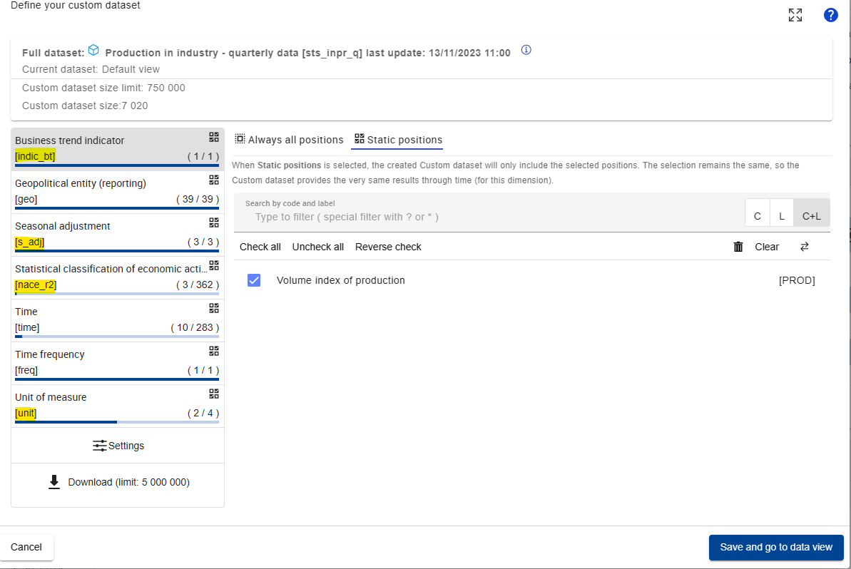
To identify the correct data, we now need to click through the different dimensions and make note of what it is that we want to use.
While the available types will vary depending on Eurostat data, most variables relevant for the OSEM Model will include:
Some variable that indicates the specific variable name, like
na_itemorindic_bt, depending on the Eurostat guidelines associated with the data collection method used.timegeo: the geography that the data belongs to (see Glossary:Country codes - Statistics Explained (europa.eu) for more information on the format).unit: the unit of the variable like €, tonnes, %, etc. (frequently also some kind of indices likeI15forIndex = 2015). This corresponds to the unit column in the Dictionary dict.s_adj: Seasonal Adjustment, e.g. NSA refers to “No Seasonal Adjustment”-
Sometimes the data we consider can be broken down even further, e.g. according to sectors or physical quantities (like different greenhouse gases). These include for example things like:
nace_r2: A column and indicator that indicates the sector according to the Statistical classification of economic activities in the European Community (NACE Revision 2)cp2_1: A column and indicator that indicates the Statistical classification of products by activity, 2.1 (CPA 2.1)siec: Standard International Energy Product Classification
Based on all the information above, let’s say that we want to add a
variable from the dataset sts_inpr_q:
industrial production,
that spans all NACE rev. 2 sectors in the sectors B to D,
for Austria,
using the unit of an index that is set to the 2015 value and
is not seasonally adjusted.
Checking the new variable
Given this information, let’s try to download it first - using the
get_eurostat function from the {eurostat}
package:
dat_raw <- get_eurostat(id = "sts_inpr_q")Now let’s filter this raw dataset down to the data series that we need:
dat_raw %>%
  filter(indic_bt == "PRD", # for industrial production variable
         nace_r2 == "B-D", # to select all NACE rev 2 sectors in B, C, and D
         s_adj == "NSA", # to get the raw, non-adjusted data
         unit == "I15", # to get the 2015 Index
         geo == "AT" # to get only the Austrian data
         ) -> dat_AT
dat_AT
This looks quite good. We can plot this really quickly:
ggplot(dat_AT, aes(x = TIME_PERIOD, y = values, color = indic_bt)) +
  geom_line(linewidth = 1) +

  # add some styling
  geom_hline(aes(yintercept = 0)) + # to get a line through 0
  labs(title = "Industrial Production in Austria", x = NULL, y = "Industrial Production Index, 2015 = 100") +
  theme_minimal(base_size = 15)+
  theme(legend.position = "bottom")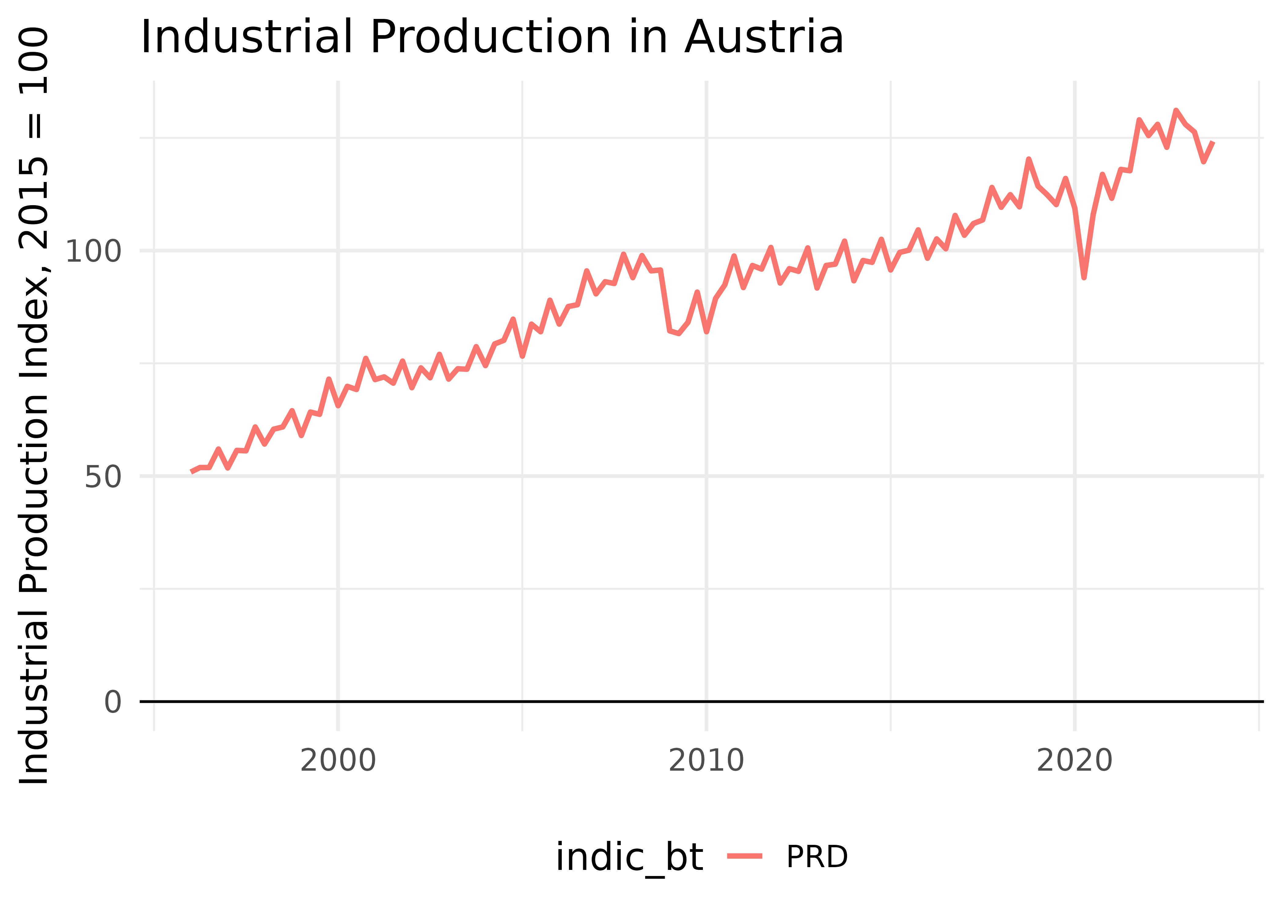
Adding the variable to the dictionary
Now that we know what the data looks like and have verified that this is what we want to add, we can add this to the dictionary. For this, we consider the column names of the dictionary again.
dict %>% names
#>  [1] "model_varname"
#>  [2] "full_name"
#>  [3] "variable_code"
#>  [4] "database"
#>  [5] "dataset_id"
#>  [6] "var_col"
#>  [7] "freq"
#>  [8] "geo"
#>  [9] "unit"
#> [10] "s_adj"
#> [11] "nace_r2"
#> [12] "cpa2_1"
#> [13] "sector"
#> [14] "direct"
#> [15] "age"
#> [16] "partner"
#> [17] "finpos"
#> [18] "p_adj"
#> [19] "meat"
#> [20] "citizen"
#> [21] "wstatus"
#> [22] "tra_oper"
#> [23] "ipcc_sector"
#> [24] "GEO"
#> [25] "Seasonal adjustment"
#> [26] "North American Industry Classification System (NAICS)"
#> [27] "North American Product Classification System (NAPCS)"
#> [28] "Prices"
#> [29] "Type of fuel"
#> [30] "Products and product groups"
#> [31] "ref_area"
#> [32] "commodity"
#> [33] "unit_measure"
And of course checking the documentation of dict again:
?dictEssentially, we need to add our new variable to our dictionary by
simply adding it as a new row. We can e.g. do this with
rbind() or bind_rows(). Depending on the
variable that we consider, we will need to fill out as many columns as
possible. For our example this means:
dict %>%
  bind_rows(tibble(
    model_varname = "IndProdIdx", # this is free to choose but must be unique
    full_name = "An index of Industrial Production",
    database  = "eurostat",
    variable_code = "PRD", # in this case use the bt_indicator information here
    dataset_id = "sts_inpr_q",
    var_col = "indic_bt", # here we specify what the column with the variables is called
    freq = "q", # for quarterly data, 'm' would be monthly
    geo = "AT",
    unit = "I15", # for index of 2015 = 100
    s_adj = "NSA", # not seasonally adjusted
    nace_r2 = "B-D")) -> new_dict
Now we are done and have successfully created a new dictionary!!
new_dict %>%
  as_tibble() %>%
  tail
#> # A tibble: 6 × 33
#>   model_varname  full_name variable_code database dataset_id var_col freq  geo
#>   <chr>          <chr>     <chr>         <chr>    <chr>      <chr>   <chr> <chr>
#> 1 CPI_Energy     Consumer… NA            statcan  18-10-000… NA      m     NA
#> 2 CPI_Gasoline   Consumer… NA            statcan  18-10-000… NA      m     NA
#> 3 IndProdPriceI… Total, I… NA            statcan  18-10-026… NA      m     NA
#> 4 IndProdGDP     Industri… NA            statcan  36-10-043… NA      m     NA
#> 5 WORLD_OIL      World Oi… NA            imf      PCPS       NA      M     NA
#> 6 IndProdIdx     An index… PRD           eurostat sts_inpr_q indic_… q     AT
#> # ℹ 25 more variables: unit <chr>, s_adj <chr>, nace_r2 <chr>, cpa2_1 <chr>,
#> #   sector <chr>, direct <chr>, age <chr>, partner <chr>, finpos <chr>,
#> #   p_adj <chr>, meat <chr>, citizen <chr>, wstatus <chr>, tra_oper <chr>,
#> #   ipcc_sector <chr>, GEO <chr>, `Seasonal adjustment` <chr>,
#> #   `North American Industry Classification System (NAICS)` <chr>,
#> #   `North American Product Classification System (NAPCS)` <chr>, Prices <chr>,
#> #   `Type of fuel` <chr>, `Products and product groups` <chr>, …
Quickly run a small model to check if it works:
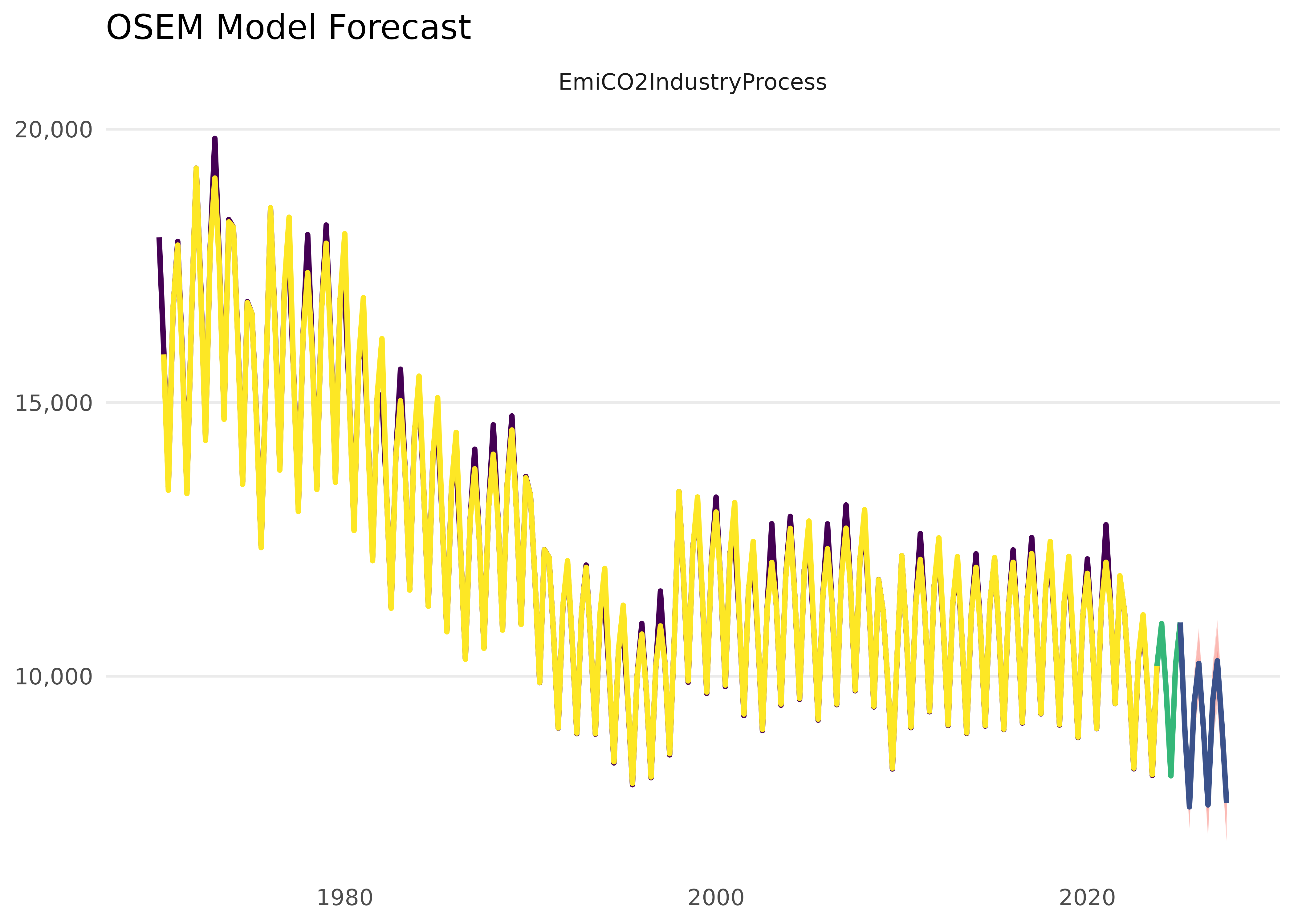
We can now put this to the test in an extremely small model. We construct a model of the CO[2] Process Emissions in Industry as a function of Gas and Electricity Prices as well as our new measure for Industrial Production:
This is then the specification that we will run. Here, the type is
set to n, which denotes an endogenously modelled
(estimated) equation. This is in contrast to d, which is
used for definitions or identities (i.e., equations that are not
estimated but are defined by relationships).
specification <- dplyr::tibble(
  type = c(
    "n"
  ),
  dependent = c(
    "EmiCO2IndustryProcess"
  ),
  independent = c(
    "HICP_Gas + HICP_Electricity + IndProdIdx"
  )
)
specification
#> # A tibble: 1 × 3
#>   type  dependent             independent
#>   <chr> <chr>                 <chr>
#> 1 n     EmiCO2IndustryProcess HICP_Gas + HICP_Electricity + IndProdIdx
With that specification set up, we now run the model using the
new_dict that we constructed earlier.
model <- run_model(specification = specification,
                   dictionary = new_dict,

                   present = FALSE,
                   quiet = TRUE,
                   constrain.to.minimum.sample = FALSE)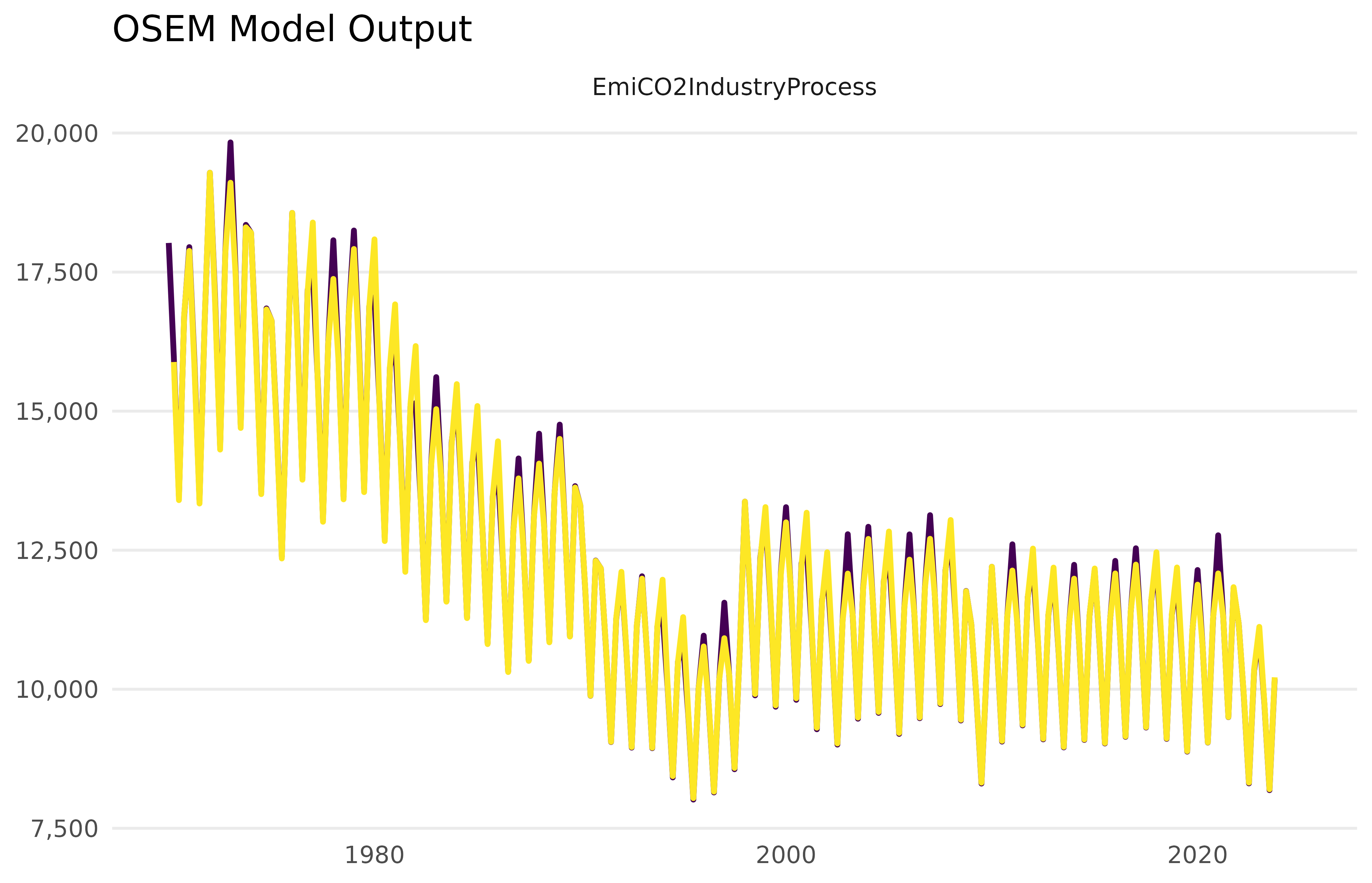
Let’s visualise this model alongside its forecast:
mod_fcast <- forecast_model(model, plot = FALSE)
#> No exogenous values provided. Model will forecast the exogenous values with an AR4 process (incl. Q dummies, IIS and SIS w 't.pval = 0.001').
#> Alternative is exog_fill_method = 'last'.
plot(mod_fcast)