Forecast OSEM model

Usage

forecast_model(
  model,
  exog_predictions = NULL,
  n.ahead = 10,
  ci.levels = c(0.5, 0.66, 0.95),
  exog_fill_method = "AR",
  ar.fill.max = 4,
  plot = TRUE,
  uncertainty_sample = 100,
  quiet = FALSE
)

Arguments

model: A model object of class 'osem'.
exog_predictions: A data.frame or tibble with values for the exogenous values. The number of rows of this data must be equal to n.ahead.
n.ahead: Periods to forecast ahead
ci.levels: Numeric vector. Vector with confidence intervals to be calculated. Default: c(0.5,0.66,0.95)
exog_fill_method: Character, either 'AR', 'auto', or 'last'. When no exogenous values have been provided, these must be inferred. When option 'exog_fill_method = "AR"' then an autoregressive model is used to further forecast the exogenous values. With 'last', simply the last available value is used. 'auto' is an auto.arima model.
ar.fill.max: Integer. When no exogenous values have been provided, these must be inferred. If option 'exog_fill_method = "AR"' then an autoregressive model is used to further forecast the exogenous values. This options determines the number of AR terms that should be used. Default is 4.
plot: Logical. Should the result be plotted? Default is TRUE.
uncertainty_sample: Integer. Number of draws to be made for the error bars. Default is 100.
quiet: Logical. Should messages about the forecast procedure be suppressed?

Value

A list of class 'osem.forecast' with the following elements:

forecast: A tibble with the forecasted values for each module.
orig_model: The original model object of class 'osem'.
dictionary: The dictionary used for the model.
exog_data: A tibble with the exogenous data used for the forecast.
exog_data_nowcast: A tibble with the exogenous data used for the nowcasting.
nowcast_data: A tibble with the nowcasted data.
args: A list with the arguments used for the forecast.
full_forecast_data: A tibble with the full forecast data, if available.

Examples

spec <- dplyr::tibble(
  type = c(
    "d",
    "d",
    "n"
  ),
  dependent = c(
    "StatDiscrep",
    "TOTS",
    "Import"
  ),
  independent = c(
    "TOTS - FinConsExpHH - FinConsExpGov - GCapitalForm - Export",
    "GValueAdd + Import",
    "FinConsExpHH + GCapitalForm"
  )
)

# \donttest{
spec <- dplyr::tibble(
 type = c(
   "d",
   "d",
   "n"
 ),
 dependent = c(
   "StatDiscrep",
   "TOTS",
   "Import"
 ),
 independent = c(
   "TOTS - FinConsExpHH - FinConsExpGov - GCapitalForm - Export",
   "GValueAdd + Import",
   "FinConsExpHH + GCapitalForm"
 )
)


a <- run_model(specification = spec,
              input = sample_input,
              primary_source = "local",
              constrain.to.minimum.sample = FALSE)
#> 
#> --- Estimation begins ---
#> Estimating Import = FinConsExpHH  +  GCapitalForm 
#> Constructing TOTS = GValueAdd  +  Import 
#> Constructing StatDiscrep = TOTS  -  FinConsExpHH  -  FinConsExpGov  -  GCapitalForm  -  Export 

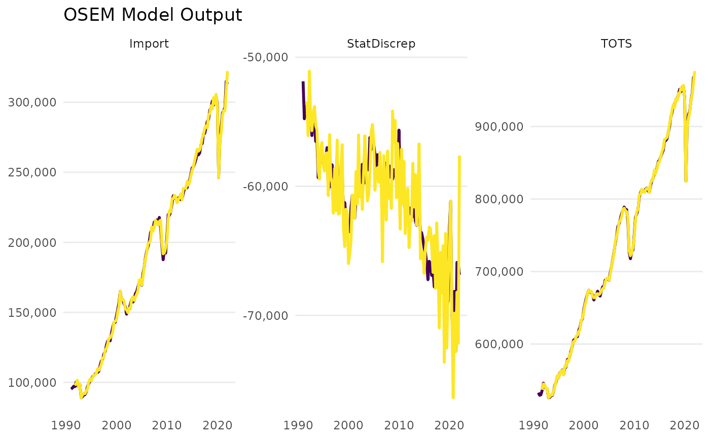forecast_model(a)
#> No exogenous values provided. Model will forecast the exogenous values with an AR4 process (incl. Q dummies, IIS and SIS w 't.pval = 0.001').
#> Alternative is exog_fill_method = 'last'.

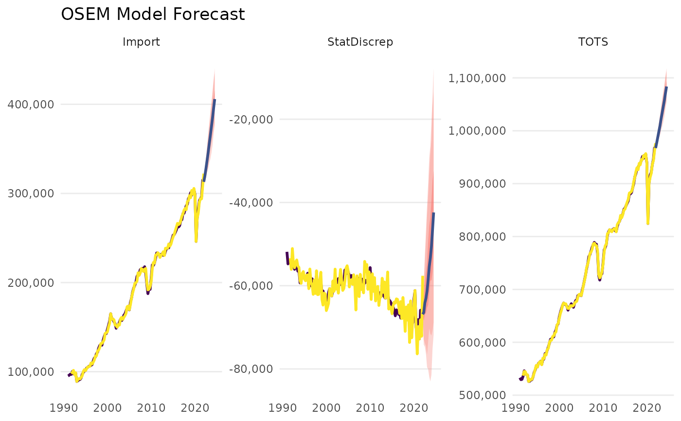#> OSEM Model Forecast Output
#> -----------------------
#> 
#> Forecast Overview:
#> Forecast Horizon: 2022-07-01 to 2024-10-01
#> Forecast Method: AR Model (Outlier and Step Shift Corrected)
#> Max AR Length: 4
#> 
#> Central Forecast Estimates: 
#> # A tibble: 10 × 4
#>    Date       Import    TOTS StatDiscrep
#>  1 2022-07-01 46750. 118296.      -8925.
#>  2 2022-10-01 47461. 120244.      -8117.
#>  3 2023-01-01 47439. 121404.      -7812.
#>  4 2023-04-01 47386. 122288.      -7748.
#>  5 2023-07-01 47720. 124005.      -7287.
#>  6 2023-10-01 47817. 125479.      -6636.
#>  7 2024-01-01 48119. 127175.      -6181.
#>  8 2024-04-01 48028. 128609.      -5880.
#>  9 2024-07-01 48208. 130441.      -5455.
#> 10 2024-10-01 48509. 132521.      -4652.


# }