11 HT5 Regression
library(tidyverse) # our main collection of functions
library(tidylog) # prints additional output from the tidyverse commands - load after tidyverse
library(haven) # allows us to load .dta (Stata specific) files
library(here) # needed to navigate to folders and files in a project
library(skimr) # allows us to get an overview over the data quickly
library(PerformanceAnalytics) # gives us a fancy correlation graph
library(broom) # to use the tidy command after a regression
#library(webr) # allows us to plot the outcome of the chi-squared test
#library(magrittr) # to use the exposition operator11.2 Data Exploration
Q: Summarize the wage variable (hrwg), years of education (yearsed), and age (age). How are wages distributed? Are age and education correlated with wages? Do the signs of the correlations make sense to you?
Using the skim() variable, we can already see a small histogram that indiciates the skew for us:
df %>%
skim()| Name | Piped data |
| Number of rows | 12670 |
| Number of columns | 9 |
| _______________________ | |
| Column type frequency: | |
| character | 4 |
| numeric | 5 |
| ________________________ | |
| Group variables | None |
Variable type: character
| skim_variable | n_missing | complete_rate | min | max | empty | n_unique | whitespace |
|---|---|---|---|---|---|---|---|
| female | 0 | 1 | 1 | 1 | 0 | 2 | 0 |
| educ | 0 | 1 | 1 | 1 | 0 | 4 | 0 |
| race | 42 | 1 | 1 | 1 | 0 | 7 | 0 |
| married | 0 | 1 | 1 | 1 | 0 | 2 | 0 |
Variable type: numeric
| skim_variable | n_missing | complete_rate | mean | sd | p0 | p25 | p50 | p75 | p100 | hist |
|---|---|---|---|---|---|---|---|---|---|---|
| age | 0 | 1 | 39.84 | 12.25 | 17.00 | 30.00 | 40.00 | 50.00 | 64.00 | ▆▇▇▇▅ |
| earnwt | 0 | 1 | 12596.62 | 1955.20 | 6592.87 | 11393.38 | 12344.94 | 13596.19 | 33593.57 | ▆▇▁▁▁ |
| yearsed | 0 | 1 | 13.43 | 2.91 | 3.00 | 12.00 | 13.00 | 16.00 | 19.00 | ▁▂▆▇▇ |
| hrwg | 0 | 1 | 22.87 | 18.36 | 3.20 | 10.70 | 17.00 | 28.25 | 269.23 | ▇▁▁▁▁ |
| lnhrwg | 0 | 1 | 2.90 | 0.64 | 1.16 | 2.37 | 2.83 | 3.34 | 5.60 | ▁▇▆▂▁ |
We also note that the race dummy is read as a character variable - indeed it contains a label and a numeric value in Stata. We can access both information using the haven package, which we used to read the data in the first place. We get the labels using as_factor() and could get the numeric information using as.numeric().
Let’s fix that - note that we do not keep the numeric information. Generally using this numeric information not a good idea!! We need an ordinal information to use correlations and other calculations - how the person who put togehter the dataset ordered the race variable can in no way indicate a rank - and let’s be glad it doesn’t).
mutate: converted 'race' from double to factor (0 new NA)
# the equivalent for the numeric information would be. But here commented out!
# df %>%
#   mutate(race = as.numeric(race)) -> df
To consider the correlations, we must first get rid of all non-numeric variables (in this case race) and can then either use the simple cor() command.
select: dropped one variable (race) age earnwt female educ yearsed
age 1.00000000 -0.20453643 0.01684272 0.08808906 0.08367609
earnwt -0.20453643 1.00000000 -0.22660452 -0.02840408 -0.03521543
female 0.01684272 -0.22660452 1.00000000 0.08966000 0.08341867
educ 0.08808906 -0.02840408 0.08966000 1.00000000 0.93478542
yearsed 0.08367609 -0.03521543 0.08341867 0.93478542 1.00000000
hrwg 0.23399072 -0.03615194 -0.10092853 0.43001863 0.44000550
lnhrwg 0.28948758 -0.03939616 -0.10509011 0.51022940 0.51801114
married 0.33321641 -0.06032386 -0.07250906 0.01641963 0.01654553
hrwg lnhrwg married
age 0.23399072 0.28948758 0.33321641
earnwt -0.03615194 -0.03939616 -0.06032386
female -0.10092853 -0.10509011 -0.07250906
educ 0.43001863 0.51022940 0.01641963
yearsed 0.44000550 0.51801114 0.01654553
hrwg 1.00000000 0.90942695 0.15782348
lnhrwg 0.90942695 1.00000000 0.18906790
married 0.15782348 0.18906790 1.00000000We could automate this using a where() command and then a logical statement:
select: dropped one variable (race) age earnwt female educ yearsed
age 1.00000000 -0.20453643 0.01684272 0.08808906 0.08367609
earnwt -0.20453643 1.00000000 -0.22660452 -0.02840408 -0.03521543
female 0.01684272 -0.22660452 1.00000000 0.08966000 0.08341867
educ 0.08808906 -0.02840408 0.08966000 1.00000000 0.93478542
yearsed 0.08367609 -0.03521543 0.08341867 0.93478542 1.00000000
hrwg 0.23399072 -0.03615194 -0.10092853 0.43001863 0.44000550
lnhrwg 0.28948758 -0.03939616 -0.10509011 0.51022940 0.51801114
married 0.33321641 -0.06032386 -0.07250906 0.01641963 0.01654553
hrwg lnhrwg married
age 0.23399072 0.28948758 0.33321641
earnwt -0.03615194 -0.03939616 -0.06032386
female -0.10092853 -0.10509011 -0.07250906
educ 0.43001863 0.51022940 0.01641963
yearsed 0.44000550 0.51801114 0.01654553
hrwg 1.00000000 0.90942695 0.15782348
lnhrwg 0.90942695 1.00000000 0.18906790
married 0.15782348 0.18906790 1.00000000But let’s consider something a bit fancier as well:
df %>%
  select(where(is.numeric)) %>%
  chart.Correlation()
select: dropped one variable (race)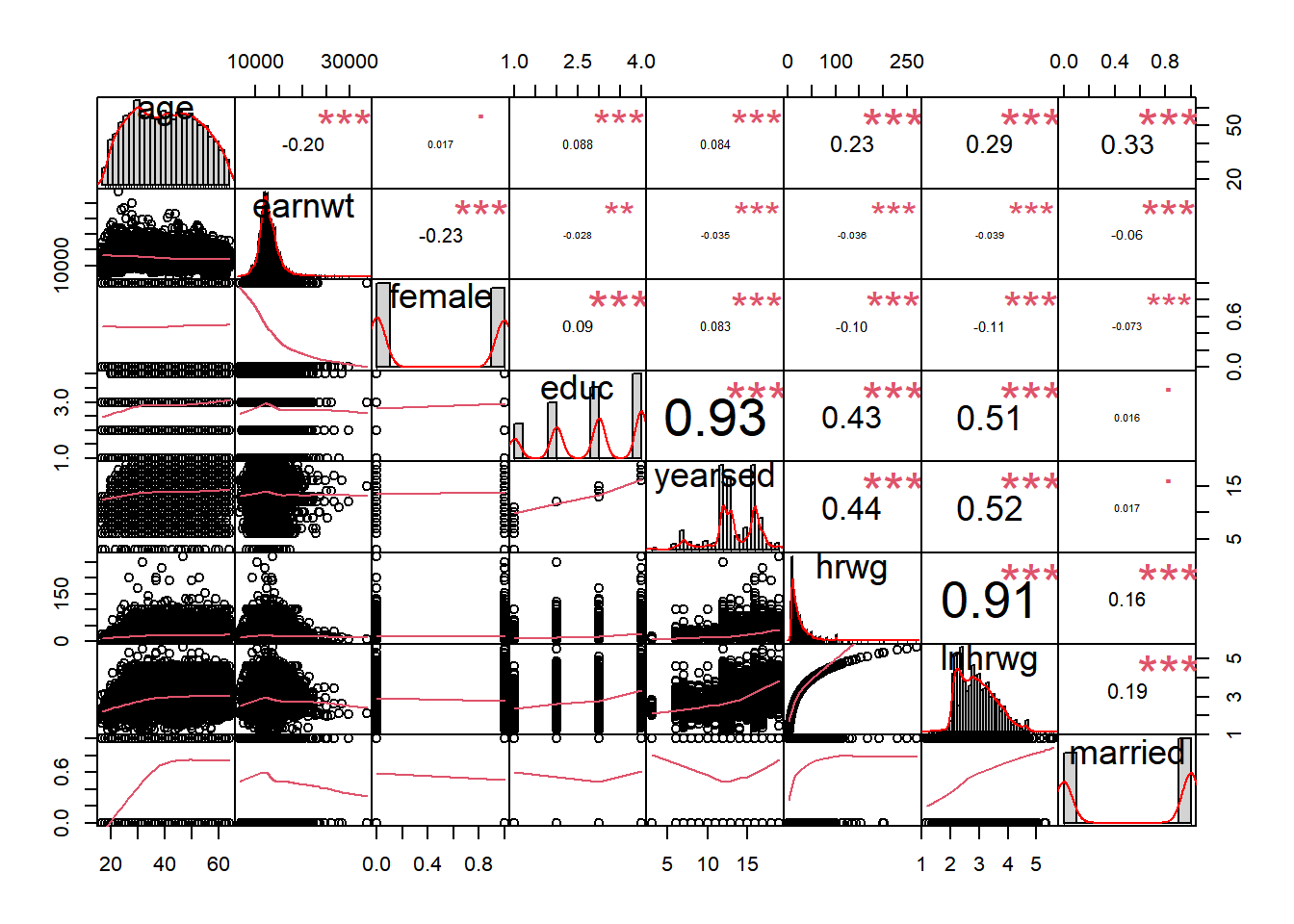
Unsurprisingly we get the strongest correlations with the education and the years of education variables as well as between the hourly wage and its logged form (hrwg and lnhrwg).
11.3 Histogram of hourly wage
We now plot a histogram of hourly wage to see the distribution. Remember, you can always use esquisser() to help with plotting (@see(plotting)).
df %>%
  ggplot() +
  aes(x = hrwg) +
  geom_histogram(fill = "orange") +

  # styling
  theme_minimal()+
  labs(title = "Histogram of hourly Wage", x = "Hourly Wage in US$")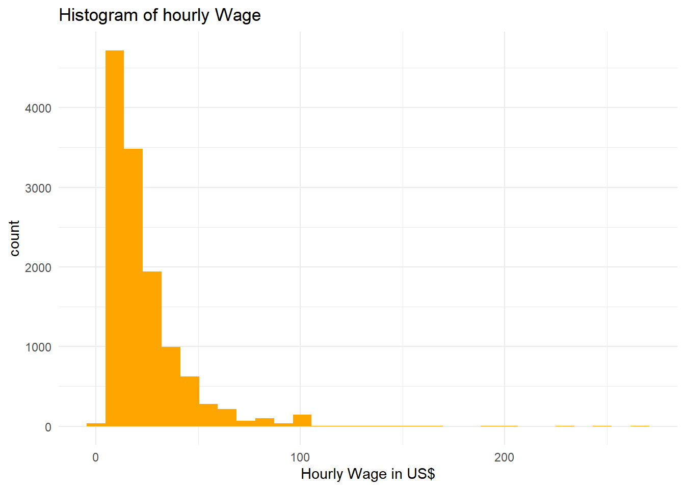
We now plot a histogram of the natural log of hourly wage:
df %>%
  ggplot() +
  aes(x = lnhrwg) +
  geom_histogram(fill = "lightblue") +

  # styling
  theme_minimal()+
labs(title = "Histogram of Log hourly Wage", x = "Log Hourly Wage in US$") 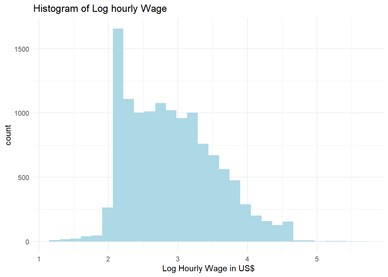
Does it look very different? What do you think is the cause of the large spike in the distribution towards the lower tail?
11.4 Simple Linear Regression
We now simply use the lm() command for the first time, which stands for “Linear Model.” Especially insteresting for us is the formula part of the lm() function, which always needs a ~ operator. An expression of the form y ~ x is interpreted as a specification that the dependent variable y is modelled by one linear predictor specified symbolically by x.
ourmodel <- lm(formula = lnhrwg ~ age + yearsed, data = df)The model result of an lm() command is not very nice to read:
ourmodel
Call:
lm(formula = lnhrwg ~ age + yearsed, data = df)

Coefficients:
(Intercept)          age      yearsed
    0.92268      0.01295      0.10916
So we typically always use the summary() command:
summary(ourmodel)
Call:
lm(formula = lnhrwg ~ age + yearsed, data = df)

Residuals:
     Min       1Q   Median       3Q      Max
-2.17099 -0.35468 -0.03062  0.33007  2.87441

Coefficients:
             Estimate Std. Error t value Pr(>|t|)
(Intercept) 0.9226840  0.0257189   35.88   <2e-16 ***
age         0.0129499  0.0003815   33.95   <2e-16 ***
yearsed     0.1091639  0.0016030   68.10   <2e-16 ***
---
Signif. codes:  0 '***' 0.001 '**' 0.01 '*' 0.05 '.' 0.1 ' ' 1

Residual standard error: 0.524 on 12667 degrees of freedom
Multiple R-squared:  0.3293,    Adjusted R-squared:  0.3292
F-statistic:  3110 on 2 and 12667 DF,  p-value: < 2.2e-16
Fantastic. See here for a step-by-step guide on what each line of this output means.
11.5 Regression with potential work experience
We need to create a variable that is called: ptexp and should look like this: age – 6 – yearsed.
Generate this variable and include it in the above regression model.
We will create this variable using our standard mutate() command and then actually pass the data directly into our lm model to show you how this is done!
df %>%
  mutate(ptexp = age - 6 - yearsed) %>%

  lm(formula = lnhrwg ~ age + yearsed + ptexp) %>%

  summary()
Call:
lm(formula = lnhrwg ~ age + yearsed + ptexp, data = .)

Residuals:
     Min       1Q   Median       3Q      Max
-2.17099 -0.35468 -0.03062  0.33007  2.87441

Coefficients: (1 not defined because of singularities)
             Estimate Std. Error t value Pr(>|t|)
(Intercept) 0.9226840  0.0257189   35.88   <2e-16 ***
age         0.0129499  0.0003815   33.95   <2e-16 ***
yearsed     0.1091639  0.0016030   68.10   <2e-16 ***
ptexp              NA         NA      NA       NA
---
Signif. codes:  0 '***' 0.001 '**' 0.01 '*' 0.05 '.' 0.1 ' ' 1

Residual standard error: 0.524 on 12667 degrees of freedom
Multiple R-squared:  0.3293,    Adjusted R-squared:  0.3292
F-statistic:  3110 on 2 and 12667 DF,  p-value: < 2.2e-16
Do you notice something strange? Why are you not able to include this variable in the regression?
11.6 Relationship between wage and age
Compute the average wage for each age. To do it by each age, we can use the group_by() command and then the summarise() command. We do not need the usual na.rm = TRUE because the hrwg variable does not contain any missing values, but it wouldn’t hurt to use it anyway:
group_by: one grouping variable (age)summarise: now 48 rows and 2 columns, ungrouped# A tibble: 48 x 2
age avg_hrwg
<dbl> <dbl>
1 17 8.63
2 18 9.35
3 19 9.41
4 20 10.3
5 21 10.5
6 22 11.8
7 23 13.7
8 24 15.2
9 25 16.5
10 26 18.0
# ... with 38 more rowsDoes it look like the relationship between the two variables is linear or non-linear? Does that seem like an intuitive result to you?
Let’s now plot this relationship:
df %>%
ggplot() +
aes(x = age, y = hrwg) +
geom_point() +
# styling
theme_minimal() +
labs(title = "Relationship between Age and Wages",x = "Age", y = "Hourly Wages")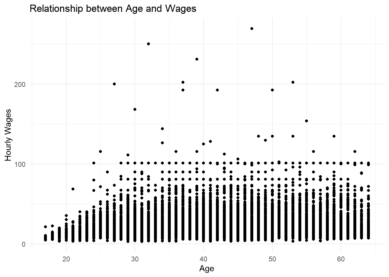
Or we can also plot the average values and add a line of the same points:
df %>%
  group_by(age) %>%
summarise(avg_hrwg = mean(hrwg)) %>%
ggplot() +
aes(x = age, y = avg_hrwg) +
geom_point(color = "blue", size = 2) +
geom_line(color = "red")+
# styling
theme_minimal() +
labs(title = "Relationship between Age and Average Wages",x = "Age", y = "Average Hourly Wages")group_by: one grouping variable (age)summarise: now 48 rows and 2 columns, ungrouped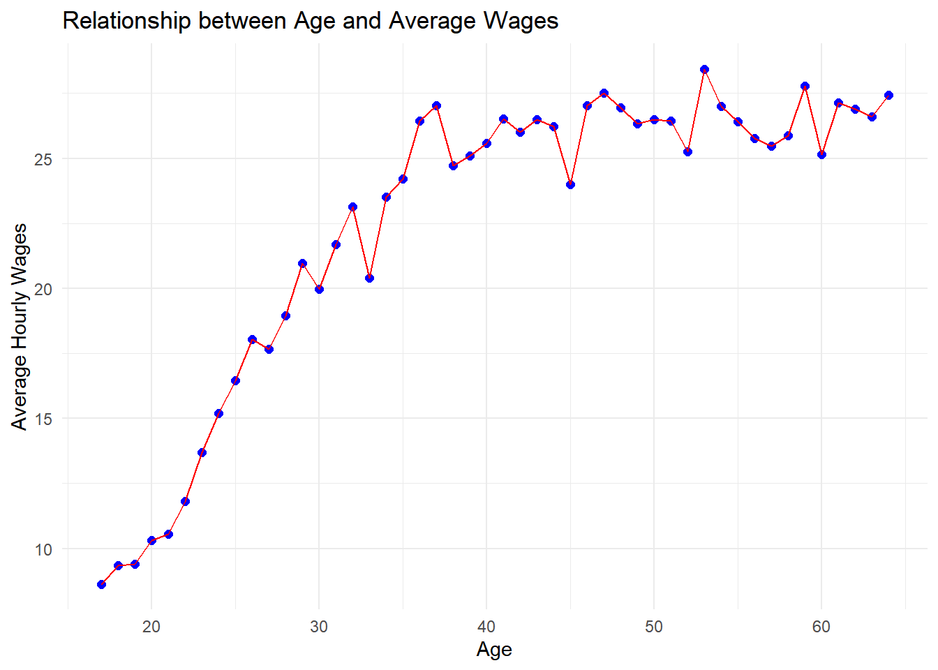
11.7 Using a non-linear age variable
We can either create an age variable before we get started using:
df %>%
  mutate(age2 = age * age) # or also age^2
mutate: new variable 'age2' (double) with 48 unique values and 0% NA# A tibble: 12,670 x 10
age earnwt female educ yearsed race hrwg lnhrwg married age2
<dbl> <dbl> <dbl+lb> <dbl+lb> <dbl> <fct> <dbl> <dbl> <dbl+lb> <dbl>
1 34 15071. 0 [male] 1 [less~ 7 6-Hi~ 10 2.30 1 [marr~ 1156
2 58 12748. 1 [fema~ 4 [coll~ 16 1-Wh~ 33.5 3.51 1 [marr~ 3364
3 49 10104. 1 [fema~ 1 [less~ 10 6-Hi~ 8 2.08 1 [marr~ 2401
4 48 14287. 0 [male] 1 [less~ 10 6-Hi~ 10 2.30 1 [marr~ 2304
5 61 10770. 0 [male] 4 [coll~ 16 1-Wh~ 20.8 3.03 1 [marr~ 3721
6 63 9866. 1 [fema~ 3 [some~ 15 1-Wh~ 22.6 3.12 1 [marr~ 3969
7 46 12702. 0 [male] 4 [coll~ 16 1-Wh~ 19.2 2.96 1 [marr~ 2116
8 48 11009. 1 [fema~ 4 [coll~ 16 1-Wh~ 25.6 3.24 1 [marr~ 2304
9 17 11480. 1 [fema~ 2 [HS] 12 1-Wh~ 9 2.20 0 [not ~ 289
10 19 12479. 1 [fema~ 3 [some~ 13 1-Wh~ 8 2.08 0 [not ~ 361
# ... with 12,660 more rowsOr we can do this directly in the lm command using the I() command, which handles a number of interactions:
Call:
lm(formula = lnhrwg ~ age + I(age^2) + yearsed, data = .)

Residuals:
     Min       1Q   Median       3Q      Max
-2.20249 -0.33198 -0.02509  0.31990  2.81432

Coefficients:
              Estimate Std. Error t value Pr(>|t|)
(Intercept) -1.103e-01  5.210e-02  -2.116   0.0343 *
age          7.057e-02  2.570e-03  27.454   <2e-16 ***
I(age^2)    -7.145e-04  3.153e-05 -22.657   <2e-16 ***
yearsed      1.076e-01  1.573e-03  68.377   <2e-16 ***
---
Signif. codes:  0 '***' 0.001 '**' 0.01 '*' 0.05 '.' 0.1 ' ' 1

Residual standard error: 0.5137 on 12666 degrees of freedom
Multiple R-squared:  0.3555,    Adjusted R-squared:  0.3553
F-statistic:  2329 on 3 and 12666 DF,  p-value: < 2.2e-16
11.8 Average Wage for Years of Schooling
compute the average wage for each year of schooling and we also add the standard deviation for each year to this!
group_by: one grouping variable (yearsed)summarise: now 15 rows and 3 columns, ungrouped# A tibble: 15 x 3
yearsed avg_hrwg sd_hrwg
<dbl> <dbl> <dbl>
1 3 10.3 2.48
2 6 12.2 8.80
3 7 11.6 6.31
4 8 11.4 4.77
5 9 12.6 6.94
6 10 11.8 7.54
7 11 11.9 6.11
8 12 16.9 11.6
9 13 18.6 13.1
10 14 21.8 14.5
11 15 21.9 13.7
12 16 30.5 20.6
13 17 39.2 22.8
14 18 47.2 28.3
15 19 44.7 29.6 And we plot this again, but first we need to do a bit of data wrangling to get the data into the right shape for our plot:
df %>%
  group_by(yearsed) %>%
  summarise(avg_hrwg = mean(hrwg),
sd_hrwg = sd(hrwg)) %>%
# this reshapes the data - we need this to use facet_wrap below
pivot_longer(-yearsed, names_to = "name", values_to = "value") %>%
# creates a factor variable that has labels, which we want to show up below side-by-side
mutate(name = factor(name, levels = c("avg_hrwg", "sd_hrwg"),
labels = c("Average Wage","Standard Deviation of Wage"))) -> df_ready_to_plotgroup_by: one grouping variable (yearsed)summarise: now 15 rows and 3 columns, ungroupedpivot_longer: reorganized (avg_hrwg, sd_hrwg) into (name, value) [was 15x3, now 30x3]mutate: converted 'name' from character to factor (0 new NA)
df_ready_to_plot# A tibble: 30 x 3
yearsed name value
<dbl> <fct> <dbl>
1 3 Average Wage 10.3
2 3 Standard Deviation of Wage 2.48
3 6 Average Wage 12.2
4 6 Standard Deviation of Wage 8.80
5 7 Average Wage 11.6
6 7 Standard Deviation of Wage 6.31
7 8 Average Wage 11.4
8 8 Standard Deviation of Wage 4.77
9 9 Average Wage 12.6
10 9 Standard Deviation of Wage 6.94
# ... with 20 more rowsNow that it is ready, we can use it to plot:
df_ready_to_plot %>%
  ggplot() +
  aes(x = yearsed, y = value) +
  geom_point(color = "blue", size = 2) +
  geom_line(color = "red") +

  geom_hline(aes(yintercept = 0)) + # we add a horizontal line at 0

  # this puts both variables side-to-side
  facet_wrap(~name) +

  # optional styling
  theme_minimal() +
  scale_y_continuous(labels = scales::dollar) + # Adds a dollar sign to the y-axis
  labs(title = "Hourly wage by Years of Education",
       subtitle = "Mean and Standard Deviation",
       x = "Yeas of Education",
       y = "Hourly Wage")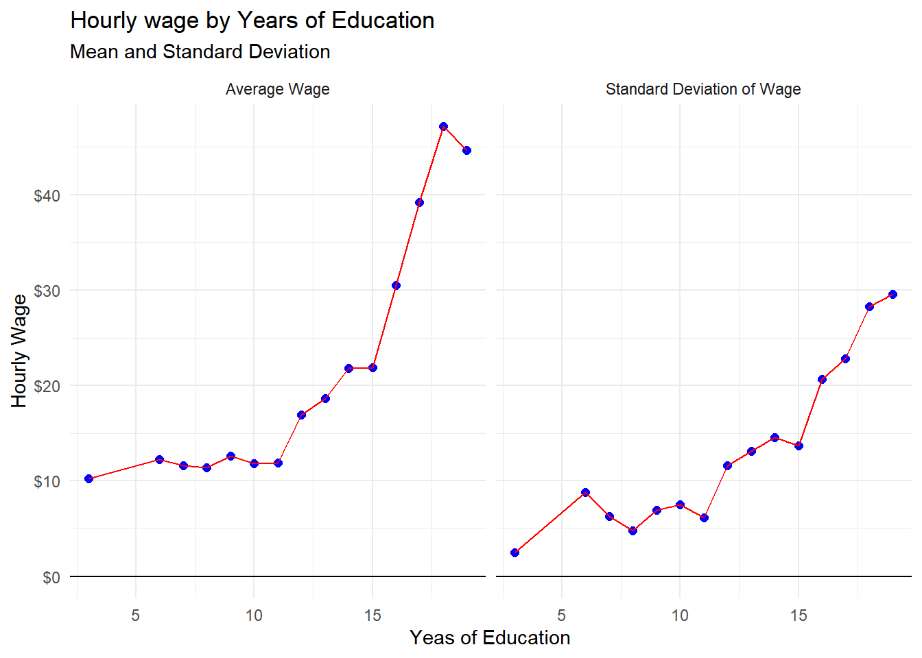
11.9 Output the resuls
Being able to present the results effectively and neatly is part of being a good researcher.
We will now consider a few options to output our regression results:
The easiest way of “cleaning” our results, is by using the tidy() function of the broom() package, which transforms our regression results from:
Call:
lm(formula = lnhrwg ~ age + I(age^2) + yearsed, data = .)

Residuals:
     Min       1Q   Median       3Q      Max
-2.20249 -0.33198 -0.02509  0.31990  2.81432

Coefficients:
              Estimate Std. Error t value Pr(>|t|)
(Intercept) -1.103e-01  5.210e-02  -2.116   0.0343 *
age          7.057e-02  2.570e-03  27.454   <2e-16 ***
I(age^2)    -7.145e-04  3.153e-05 -22.657   <2e-16 ***
yearsed      1.076e-01  1.573e-03  68.377   <2e-16 ***
---
Signif. codes:  0 '***' 0.001 '**' 0.01 '*' 0.05 '.' 0.1 ' ' 1

Residual standard error: 0.5137 on 12666 degrees of freedom
Multiple R-squared:  0.3555,    Adjusted R-squared:  0.3553
F-statistic:  2329 on 3 and 12666 DF,  p-value: < 2.2e-16
to this:
# A tibble: 4 x 5
term estimate std.error statistic p.value
<chr> <dbl> <dbl> <dbl> <dbl>
1 (Intercept) -0.110 0.0521 -2.12 3.43e- 2
2 age 0.0706 0.00257 27.5 3.10e-161
3 I(age^2) -0.000714 0.0000315 -22.7 1.92e-111
4 yearsed 0.108 0.00157 68.4 0. This does not yet look very nice - but is actually very helpful in working with regression model output and indeed saving this is really easy:
df %>%
  lm(formula = lnhrwg ~ age + I(age^2) + yearsed) %>%
tidy() %>%
write_csv(here("output","regressionoutput.csv"))So let’s try some styling now. For this, we can use a few nice packages.
Let’s start with stargazer(), which can output extremely helpful LaTeX (default) or html code. Let’s create some text output first though, using the type = "text"
library(stargazer)
df %>%
  lm(formula = lnhrwg ~ age + I(age^2) + yearsed) %>%
  stargazer(type = "text")
================================================
                        Dependent variable:
                    ----------------------------
                               lnhrwg
------------------------------------------------
age                           0.071***
                              (0.003)

I(age2)                      -0.001***
                             (0.00003)

yearsed                       0.108***
                              (0.002)

Constant                      -0.110**
                              (0.052)

------------------------------------------------
Observations                   12,670
R2                             0.355
Adjusted R2                    0.355
Residual Std. Error      0.514 (df = 12666)
F Statistic         2,328.522*** (df = 3; 12666)
================================================
Note:                *p<0.1; **p<0.05; ***p<0.01
You can simply save the output of this using the option out:
df %>%
  lm(formula = lnhrwg ~ age + I(age^2) + yearsed) %>%
  stargazer(type = "text", out = here("output","regressiontable.txt"))
If you work in RMarkdown (and I suggest you do), there are some other nice ways of styling and outputting your results, namely the package kableExtra, which you can check out here and here.
You could also use the gtsummary package (see here), which has a handy function named tbl_regression(), but it needs the age2 variable to be created before the lm() command:
library(gtsummary)
df %>%
  mutate(age2 = age^2) %>%
  lm(formula = lnhrwg ~ age + age2 + yearsed) %>%
tbl_regression(intercept = TRUE)| Characteristic | Beta | 95% CI1 | p-value |
|---|---|---|---|
| (Intercept) | -0.11 | -0.21, -0.01 | 0.034 |
| Age | 0.07 | 0.07, 0.08 | <0.001 |
| Age | 0.00 | 0.00, 0.00 | <0.001 |
| total years of education | 0.11 | 0.10, 0.11 | <0.001 |
|
1
CI = Confidence Interval
|
|||
Yet another alternative is coming from the jtools package (see here).
library(jtools)
df %>%
  lm(formula = lnhrwg ~ age + I(age^2) + yearsed) %>%
  export_summs()
Warning in checkMatrixPackageVersion(): Package version inconsistency detected.
TMB was built with Matrix version 1.2.18
Current Matrix version is 1.3.2
Please re-install 'TMB' from source using install.packages('TMB', type = 'source') or ask CRAN for a binary version of 'TMB' matching CRAN's 'Matrix' package| Model 1 | |
|---|---|
| (Intercept) | -0.11 * |
| (0.05) | |
| age | 0.07 *** |
| (0.00) | |
| I(age^2) | -0.00 *** |
| (0.00) | |
| yearsed | 0.11 *** |
| (0.00) | |
| N | 12670 |
| R2 | 0.36 |
| *** p < 0.001; ** p < 0.01; * p < 0.05. | |
Again you can save your table using the options to.file where you can use the arguments “Word” or “docx” (equivalent), “pdf,” “html,” or “xlsx” together with the file.name argument.