7 HT1 Probability
7.1 Part 1
series <- c(0, 1, 6, 3, 5, 8, 6, 7, 8, 9, 10, 4, 12, 0, 14, 1, 9, 3, 4, 5, 6, 7, 2, 4, 16)Order the series using the sort() command.
ordered_series <- sort(series)
table(series)series
0 1 2 3 4 5 6 7 8 9 10 12 14 16
2 2 1 2 3 2 3 2 2 2 1 1 1 1 [1] [0,4) [0,4) [4,8) [0,4) [4,8) [8,12) [4,8) [4,8)
[9] [8,12) [8,12) [8,12) [4,8) [12,16] [0,4) [12,16] [0,4)
[17] [8,12) [0,4) [4,8) [4,8) [4,8) [4,8) [0,4) [4,8)
[25] [12,16]
Levels: [0,4) [4,8) [8,12) [12,16]
tibble(series = cut(series, breaks = seq(0,20,4),right = FALSE, include.lowest = TRUE,labels = FALSE)) %>%
  ggplot() +
  aes(x=series)+
  geom_histogram()
`stat_bin()` using `bins = 30`. Pick better value with `binwidth`.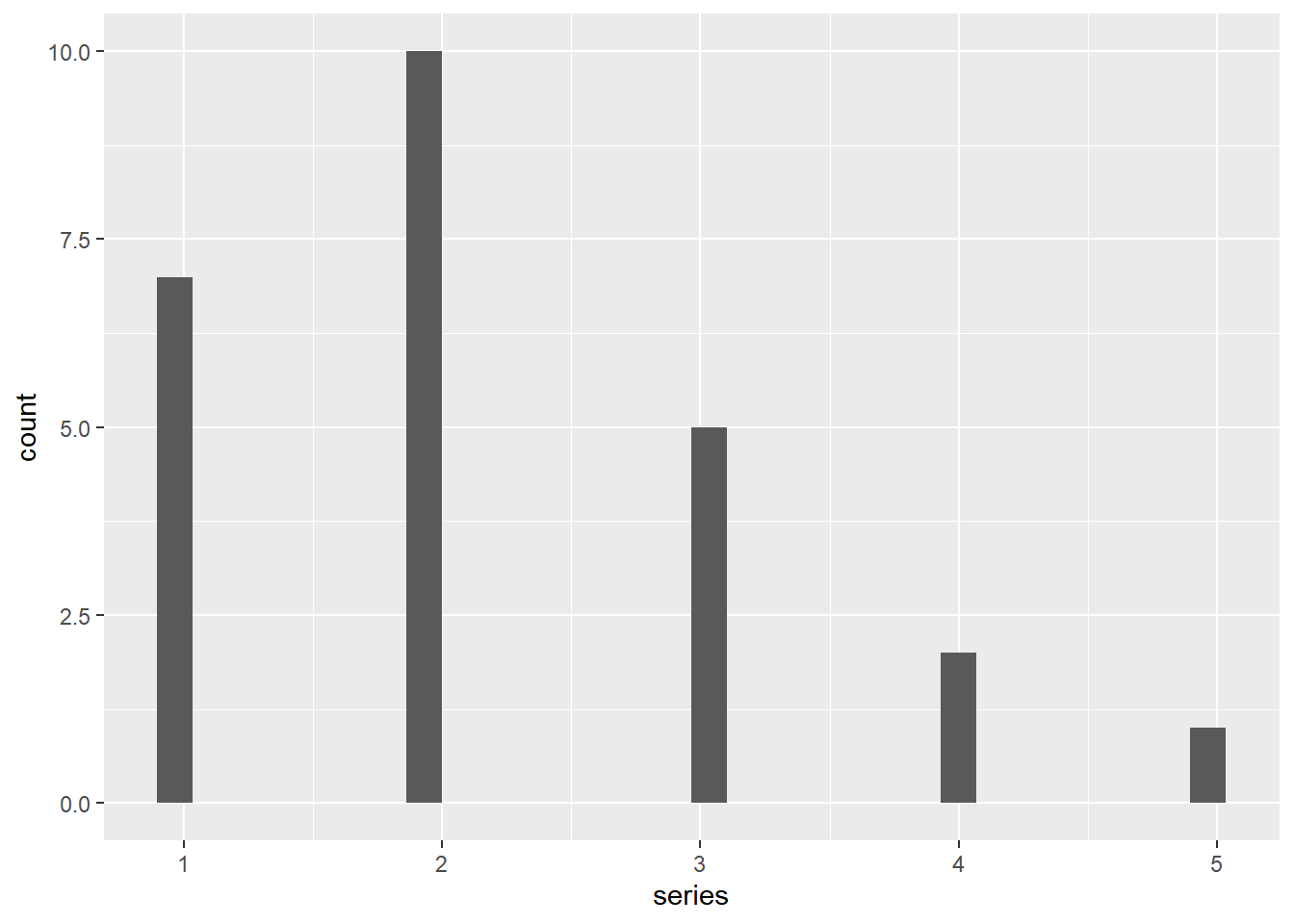
Mode(series)[1] 4 6
attr(,"freq")
[1] 3
Median(series)[1] 6
Mean(series)[1] 67.1.1 Percentiles
The formula for any percentile is:
\[ \frac{(n+1)*P}{100} \]
[1] 19.50 10.40 5.98This means those values are, rounding to the nearest integer:
positions <- round(percentile_ranks)
ordered_series[positions]
[1] 9 4 3Using a percentile function:
75% 40% 23%
8.0 4.6 3.0 75% 40% 23%
8.0 4.5 3.0 We see that it depends on the algorith!
7.1.2 Range
range(series)[1] 0 16
sd(series)[1] 4.153312
var(series)[1] 17.25
IQR(series)[1] 5
quantile(series,type = 6) 0% 25% 50% 75% 100%
0.0 3.0 6.0 8.5 16.0 7.1.3 Weighted Mean
weighted.mean(x = c(6,4),
              w = c(25,50))
[1] 4.666667
6*25/75 + 4*50/75[1] 4.6666677.2 Part 2
Let’s load some more libraries:
library(haven) # allows us to load .dta (Stata specific) files
library(here) # needed to navigate to folders and files in a project
Load the dataset:
7.2.1 Number of countries in the data
Given that we know the dataset, we can just use the number of observations (rows):
nrow(df)[1] 193But to be more accurate:
distinct: no rows removed[1] 1937.2.2 What types of data are GDP per capita & democracy?
select: dropped 4 variables (cname, ccodealp, bl_asy25mf, wdi_trade)tibble [193 x 2] (S3: tbl_df/tbl/data.frame)
$ gle_rgdpc: num [1:193] 1155 7391 4861 28365 3998 ...
..- attr(*, "label")= chr "Real GDP per Capita (2005)"
..- attr(*, "format.stata")= chr "%9.0g"
$ chga_demo: dbl+lbl [1:193] 0, 1, 0, 1, 0, 1, 0, 1, 1, 1, 1, 0, 0, 1, 1, 1, 1...
..@ label : chr "Democracy"
..@ format.stata: chr "%15.0g"
..@ labels : Named num [1:2] 0 1
.. ..- attr(*, "names")= chr [1:2] "0. Dictatorship" "1. Democracy"
- attr(*, "label")= chr "Quality of Government Basic dataset 2015 - Cross-Section"
- attr(*, "notes")= chr [1:2] "\"I am 100% sure that we're not completely sure.\"" "1"Now we can see a lot of information - including the labels, the stata formats and the data types in R. More easily, we can access them exactly as well like this:
df$gle_rgdpc %>%
  class()
[1] "numeric"And:
df$chga_demo %>%
  class()
[1] "haven_labelled" "vctrs_vctr" "double" Now we know that democracy in R is a numeric variable (double) that is labelled. We can access those values using:
df$chga_demo %>%
  print_labels()
Labels:
 value           label
     0 0. Dictatorship
     1    1. Democracy
Or like this, when we convert it to the standard R variable that is used in such cases: a factor.
df$chga_demo %>%
  as_factor()
[1] 0. Dictatorship 1. Democracy 0. Dictatorship 1. Democracy
[5] 0. Dictatorship 1. Democracy 0. Dictatorship 1. Democracy
[9] 1. Democracy 1. Democracy 1. Democracy 0. Dictatorship
[13] 0. Dictatorship 1. Democracy 1. Democracy 1. Democracy
[17] 1. Democracy 1. Democracy 0. Dictatorship 0. Dictatorship
[21] 1. Democracy 1. Democracy 1. Democracy 0. Dictatorship
[25] 1. Democracy 0. Dictatorship 1. Democracy 0. Dictatorship
[29] 0. Dictatorship 0. Dictatorship 1. Democracy 1. Democracy
[33] 0. Dictatorship 1. Democracy 0. Dictatorship 1. Democracy
[37] 0. Dictatorship 1. Democracy 1. Democracy 1. Democracy
[41] 0. Dictatorship 0. Dictatorship 1. Democracy 1. Democracy
[45] 0. Dictatorship 1. Democracy 1. Democracy 1. Democracy
[49] 1. Democracy 1. Democracy 1. Democracy 1. Democracy
[53] 1. Democracy 0. Dictatorship 0. Dictatorship 0. Dictatorship
[57] 1. Democracy 0. Dictatorship 1. Democracy 1. Democracy
[61] 0. Dictatorship 0. Dictatorship 1. Democracy 0. Dictatorship
[65] 1. Democracy 1. Democracy 1. Democracy 1. Democracy
[69] 1. Democracy 1. Democracy 0. Dictatorship 0. Dictatorship
[73] 0. Dictatorship 1. Democracy 1. Democracy 1. Democracy
[77] 1. Democracy 1. Democracy 0. Dictatorship 0. Dictatorship
[81] 1. Democracy 1. Democracy 1. Democracy 0. Dictatorship
[85] 1. Democracy 1. Democracy 0. Dictatorship 0. Dictatorship
[89] 1. Democracy 0. Dictatorship 1. Democracy 0. Dictatorship
[93] 1. Democracy 0. Dictatorship 0. Dictatorship 0. Dictatorship
[97] 1. Democracy 1. Democracy 0. Dictatorship 1. Democracy
[101] 1. Democracy 1. Democracy 1. Democracy 1. Democracy
[105] 0. Dictatorship 1. Democracy 1. Democracy 1. Democracy
[109] 0. Dictatorship 1. Democracy 1. Democracy <NA>
[113] 1. Democracy 1. Democracy 0. Dictatorship 0. Dictatorship
[117] 0. Dictatorship 0. Dictatorship 0. Dictatorship 1. Democracy
[121] 1. Democracy 1. Democracy 1. Democracy 1. Democracy
[125] 1. Democracy 1. Democracy 1. Democracy 1. Democracy
[129] 1. Democracy 1. Democracy 1. Democracy 1. Democracy
[133] 1. Democracy 1. Democracy 1. Democracy 1. Democracy
[137] 1. Democracy 1. Democracy 1. Democracy 1. Democracy
[141] 1. Democracy 0. Dictatorship 1. Democracy 0. Dictatorship
[145] 0. Dictatorship 1. Democracy 1. Democracy 1. Democracy
[149] 1. Democracy 1. Democracy 0. Dictatorship 1. Democracy
[153] 1. Democracy 0. Dictatorship 1. Democracy 0. Dictatorship
[157] 1. Democracy 0. Dictatorship 1. Democracy 0. Dictatorship
[161] 0. Dictatorship 0. Dictatorship 1. Democracy 0. Dictatorship
[165] 1. Democracy 0. Dictatorship 1. Democracy 1. Democracy
[169] 0. Dictatorship 0. Dictatorship 1. Democracy 0. Dictatorship
[173] 0. Dictatorship 1. Democracy 0. Dictatorship 0. Dictatorship
[177] 1. Democracy 0. Dictatorship 1. Democracy 0. Dictatorship
[181] 1. Democracy 1. Democracy 0. Dictatorship 1. Democracy
[185] 0. Dictatorship 1. Democracy 0. Dictatorship 1. Democracy
[189] 0. Dictatorship 1. Democracy 0. Dictatorship 0. Dictatorship
[193] 0. Dictatorship
attr(,"label")
[1] Democracy
Levels: 0. Dictatorship 1. Democracy7.2.3 List the top-5 countries with the lowest average schooling years.
Arrange orders the data according to the argument you provide. Here we use the average schooling years bl_asy25mf.
df %>%
  arrange(bl_asy25mf) %>%
  head()
# A tibble: 6 x 6
cname ccodealp bl_asy25mf chga_demo gle_rgdpc wdi_trade
<chr> <chr> <dbl> <dbl+lbl> <dbl> <dbl>
1 Mozambique MOZ 1.20 0 [0. Dictatorship] 742. 80.1
2 Niger NER 1.44 1 [1. Democracy] 566. 71.3
3 Mali MLI 1.47 1 [1. Democracy] 946. 65.9
4 Yemen YEM 2.51 0 [0. Dictatorship] NA 65.1
5 Burundi BDI 2.68 1 [1. Democracy] 574. 48.1
6 Gambia GMB 2.79 0 [0. Dictatorship] 1455. 65.67.2.4 What is the median and mean for average schooling years?
df %>%
  summarise(schoolyears_median = median(bl_asy25mf, na.rm = TRUE),
            schoolyears_mean = mean(bl_asy25mf, na.rm = TRUE))
summarise: now one row and 2 columns, ungrouped# A tibble: 1 x 2
schoolyears_median schoolyears_mean
<dbl> <dbl>
1 8.35 7.817.2.5 Compare the average GDP per capita for democratic and non-democratic countries.
group_by: one grouping variable (chga_demo)summarise: now 3 rows and 2 columns, ungrouped# A tibble: 3 x 2
chga_demo gdp_mean
<dbl+lbl> <dbl>
1 0 [0. Dictatorship] 8803.
2 1 [1. Democracy] 14199.
3 NA 95061.If we want to print the actual values for the democracy variable, we can use the as_factor() command from the haven package again.
df %>%
  mutate(chga_demo = as_factor(chga_demo)) %>%
  group_by(chga_demo) %>%
  summarise(mean_gdp = mean(gle_rgdpc, na.rm = TRUE))
mutate: converted 'chga_demo' from double to factor (0 new NA)group_by: one grouping variable (chga_demo)summarise: now 3 rows and 2 columns, ungrouped# A tibble: 3 x 2
chga_demo mean_gdp
<fct> <dbl>
1 0. Dictatorship 8803.
2 1. Democracy 14199.
3 <NA> 95061.7.2.6 Generate a binary variable for high-skilled countries
We call the variable hskill where 1 is average schooling years greater than 12 years, and 0 otherwise:
mutate: new variable 'hskill' (double) with 3 unique values and 26% NA# A tibble: 193 x 7
cname ccodealp bl_asy25mf chga_demo gle_rgdpc wdi_trade hskill
<chr> <chr> <dbl> <dbl+lbl> <dbl> <dbl> <dbl>
1 Afghanistan AFG 3.21 0 [0. Dictat~ 1155. 55.0 0
2 Albania ALB 10.4 1 [1. Democr~ 7391. 86.3 0
3 Algeria DZA 6.83 0 [0. Dictat~ 4861. 69.9 0
4 Andorra AND NA 1 [1. Democr~ 28365. NA NA
5 Angola AGO NA 0 [0. Dictat~ 3998. 105. NA
6 Antigua an~ ATG NA 1 [1. Democr~ 11203. 104. NA
7 Azerbaijan AZE NA 0 [0. Dictat~ 9073. 75.0 NA
8 Argentina ARG 9.28 1 [1. Democr~ 12553. 40.1 0
9 Australia AUS 12.0 1 [1. Democr~ 34707. 39.5 1
10 Austria AUT 9.71 1 [1. Democr~ 34022. 104. 0
# ... with 183 more rowsBecause we want to use this later, we will save the dataset by adding -> df at the end. Here we also add the mutate(chga_demo = as_factor(chga_demo)) that we mentioned above.
df %>%
mutate(hskill = ifelse(test = bl_asy25mf > 12, 1, 0)) %>%
mutate(chga_demo = as_factor(chga_demo)) -> dfmutate: new variable 'hskill' (double) with 3 unique values and 26% NAmutate: converted 'chga_demo' from double to factor (0 new NA)7.2.7 Tabulate high-skilled countries binary variable and democracy variable
select: dropped 5 variables (cname, ccodealp, bl_asy25mf, gle_rgdpc, wdi_trade) chga_demo
hskill 0. Dictatorship 1. Democracy
0 54 81
1 0 87.2.8 What is the standard deviation for trade openness?
To summarise data again, we can use the summarise() command again:
summarise: now one row and 2 columns, ungrouped# A tibble: 1 x 2
trade_sd gdp_sd
<dbl> <dbl>
1 44.3 16090.Using a more complicated (yet more flexible) approach (don’t forget the ~ before the function and to use . for the column value, see 2.2.9).
summarise: now one row and 2 columns, ungrouped# A tibble: 1 x 2
wdi_trade gle_rgdpc
<dbl> <dbl>
1 44.3 16090.This way, we can also calculate the coefficient of variation, which is:
\[ CV = \frac{\sigma}{\mu} \]
summarise: now one row and 2 columns, ungrouped# A tibble: 1 x 2
wdi_trade gle_rgdpc
<dbl> <dbl>
1 0.496 1.28Of course we could have just calculated it manually:
df %>%
  summarise(across(.cols = c(wdi_trade, gle_rgdpc), .fns = ~sd(., na.rm = TRUE)/mean(., na.rm = TRUE)))
summarise: now one row and 2 columns, ungrouped# A tibble: 1 x 2
wdi_trade gle_rgdpc
<dbl> <dbl>
1 0.496 1.287.2.9 Create a histogram for GDP per capita with percent as the Y-axis, including the normal-density plot.
Creating the histogram is very easy:
df %>%
  ggplot() +
  aes(x = gle_rgdpc) +

  geom_histogram()
`stat_bin()` using `bins = 30`. Pick better value with `binwidth`.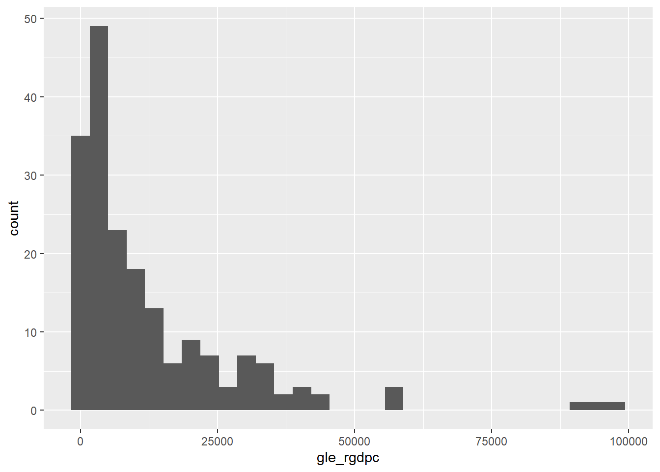
But sadly again, adding the normal distribution is slightly more difficult. I also add some styling at the bottom.
# If the ggh4x library is not installed yet, please use the line below to install:
# devtools::install_github("teunbrand/ggh4x")
library(ggh4x)

df %>%
  ggplot() +
  aes(x = gle_rgdpc) +

  # we set the binwidth, because we need it for the normal distribution function below
  geom_histogram(binwidth =  1000, fill = "darkred") +

  # This adds a line for the normal density
  stat_theodensity(aes(y=after_stat(count)*1000)) +

  # additional optional styling
  theme_minimal() +
  labs(title = "Histogram of GDP per capita",
       x = "GDP per capita",
       y = "Frequency")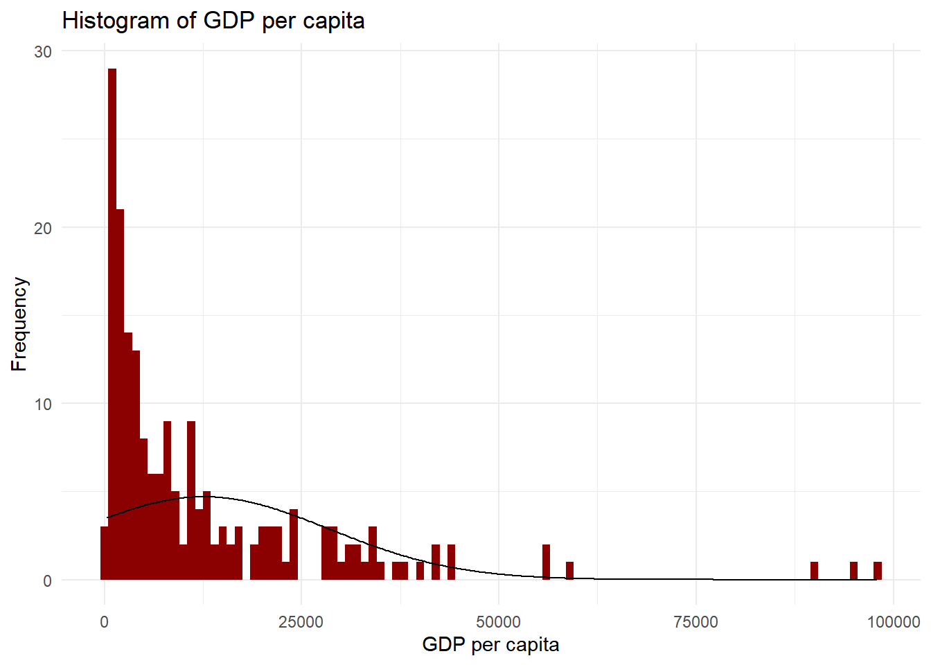
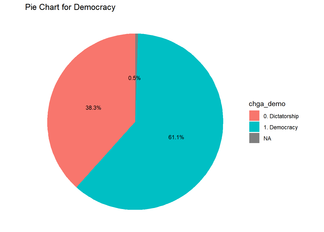
7.2.10 Pie chart for democracy
Also showing the percentage for each category including missing values.
Let’s first summarise the information we want to plot:
df %>%
  group_by(chga_demo) %>%
  count(chga_demo) %>%
  ungroup() %>%

  mutate(pct = n/sum(n)) %>%

  # We need this to put the percentage labels in the right place
  # the calculation is simply putting the label into the middle of the pie chart chunk
  arrange(desc(chga_demo)) %>%
  mutate(ypos = cumsum(pct)- 0.5*pct) %>%

  # Now we just create a nice label
  mutate(pct_label = paste0(round(pct, 3)*100,"%")) -> democracy_counts
group_by: one grouping variable (chga_demo)count: now 3 rows and 2 columns, one group variable remaining (chga_demo)ungroup: no grouping variablesmutate: new variable 'pct' (double) with 3 unique values and 0% NAmutate: new variable 'ypos' (double) with 3 unique values and 0% NAmutate: new variable 'pct_label' (character) with 3 unique values and 0% NA
democracy_counts# A tibble: 3 x 5
chga_demo n pct ypos pct_label
<fct> <int> <dbl> <dbl> <chr>
1 1. Democracy 118 0.611 0.306 61.1%
2 0. Dictatorship 74 0.383 0.803 38.3%
3 <NA> 1 0.00518 0.997 0.5% `
ggplot(democracy_counts) +
  aes(x="", y = pct, fill = chga_demo, label = pct_label) +
  geom_col() +

  coord_polar("y", start = 0) +
  geom_text(aes(y = ypos), color = "black", size=3) +

  # some styling
  theme_void() +
  labs(title = "Pie Chart for Democracy")