getspanel: Getting Started

The getspanel package can be downloaded and installed from CRAN here by simply using:

install.packages("getspanel")

The source code of the package is on GitHub and the development version can be installed using:

# install.packages("devtools")
devtools::install_github("moritzpschwarz/getspanel", ref = "devel")

Once installed we need to load the library:

library(getspanel)
library(fixest)

Currently the package is called getspanel to align with the gets package, but it’s main function of course remains the isatpanel function.

The isatpanel function implements the empirical break detection algorithm that is described in a paper by Felix Pretis and Moritz Schwarz and was applied to a study by Nico Koch and colleagues on EU Road CO₂ emissions, which was published in Nature Energy in 2022.

A quick overview over what has changed:

We can now use the function approach as well as the traditional gets approach. This means that we can specify a model using y and mxreg as well as time and id as vectors, but we can now also simply supply a data.frame and a function in the form y ~ x + z + I(x^2) to e.g. specify polynomials. This means we will then need an index argument, which specifies the
The ar argument now works
We can now use the fixest package to speed up model estimation with large i (for short panels, the default method is still faster).The package can be activated using the new engine argument.
Using the fixest package also allows us to calculate clustered standard errors.
We can now be certain that unbalanced panels would work as intended, which was not the case before.
The mxbreak and break.method arguments have been removed. Instead the function now produces the break matrix itself. This now implements the following saturation methods in a user friendly way:
iis: Impulse Indicator Saturation
jsis: Joint Step Indicator Saturation (Common Breaks over time)
csis: Coefficient Step Indicator Saturation (Common Coefficient Breaks over time)
fesis: Fixed Effect Step Indicator Saturation (Breaks in the Group Fixed Effect over time)
cfesis: Coefficient Fixed Effect Step Indicator Saturation (Breaks in the coefficient for each individual)

The isatpanel function

We first load some data of EU CO2 Emissions in the housing sector.

data("EUCO2residential")
head(EUCO2residential)
 [38;5;246m# A tibble: 6 × 9 [39m
  country  year  lgdp  lhdd  lcdd urban av.rate     pop agg.directem
   [3m [38;5;246m<chr> [39m [23m    [3m [38;5;246m<dbl> [39m [23m  [3m [38;5;246m<dbl> [39m [23m  [3m [38;5;246m<dbl> [39m [23m  [3m [38;5;246m<dbl> [39m [23m  [3m [38;5;246m<dbl> [39m [23m    [3m [38;5;246m<dbl> [39m [23m    [3m [38;5;246m<dbl> [39m [23m         [3m [38;5;246m<dbl> [39m [23m
 [38;5;250m1 [39m Austria   [4m1 [24m969  25.6     [31mNA [39m     [31mNA [39m  65.2       [31mNA [39m       [31mNA [39m            [31mNA [39m
 [38;5;250m2 [39m Austria   [4m1 [24m970  25.7     [31mNA [39m     [31mNA [39m  65.3       [31mNA [39m       [31mNA [39m            [31mNA [39m
 [38;5;250m3 [39m Austria   [4m1 [24m971  25.8     [31mNA [39m     [31mNA [39m  65.3       [31mNA [39m 7 [4m5 [24m [4m0 [24m [4m0 [24m482            [31mNA [39m
 [38;5;250m4 [39m Austria   [4m1 [24m972  25.8     [31mNA [39m     [31mNA [39m  65.3       [31mNA [39m 7 [4m5 [24m [4m4 [24m [4m4 [24m201            [31mNA [39m
 [38;5;250m5 [39m Austria   [4m1 [24m973  25.9     [31mNA [39m     [31mNA [39m  65.3       [31mNA [39m 7 [4m5 [24m [4m8 [24m [4m6 [24m115            [31mNA [39m
 [38;5;250m6 [39m Austria   [4m1 [24m974  25.9     [31mNA [39m     [31mNA [39m  65.3       [31mNA [39m 7 [4m5 [24m [4m9 [24m [4m9 [24m038            [31mNA [39m

# let's subset this a little bit to speed this up
EUCO2residential <- EUCO2residential[EUCO2residential$year > 2000 & 
                                       EUCO2residential$country %in% c("Germany", "Austria",
                                                                       "Belgium", "Italy", 
                                                                       "Sweden", "Denmark"),]

# let's create a log emissions per capita variable
EUCO2residential$lagg.directem_pc <- log(EUCO2residential$agg.directem/EUCO2residential$pop)

# and let's also turn off printing the intermediate output from isatpanel
options(print.searchoutput = FALSE)

Let’s look at how we input what we want to model. Each isatpanel command takes:

Basics

A specification of the source data, the group and time variable and the group-time characteristics. This can be entered into the function in two ways:

In the gets package style i.e. using vectors and matrices to specify y, mxreg, time and id
But also in a form that resembles the lm and plm specification i.e. inputting a data.frame (or matrix or tibble), a formula argument as well as character vectors for index (in the form c("group_variable_name", "time_variable_name"))

A an argument for the Fixed Effect Specification using effect.

This already means that the following two commands will give the same result:

Using the new method

is_lm <- isatpanel(data = EUCO2residential,
                   formula = lagg.directem_pc ~ lgdp + I(lgdp^2) + pop,
                   index = c("country","year"),
                   
                   effect = "twoways",
                   
                   fesis = TRUE)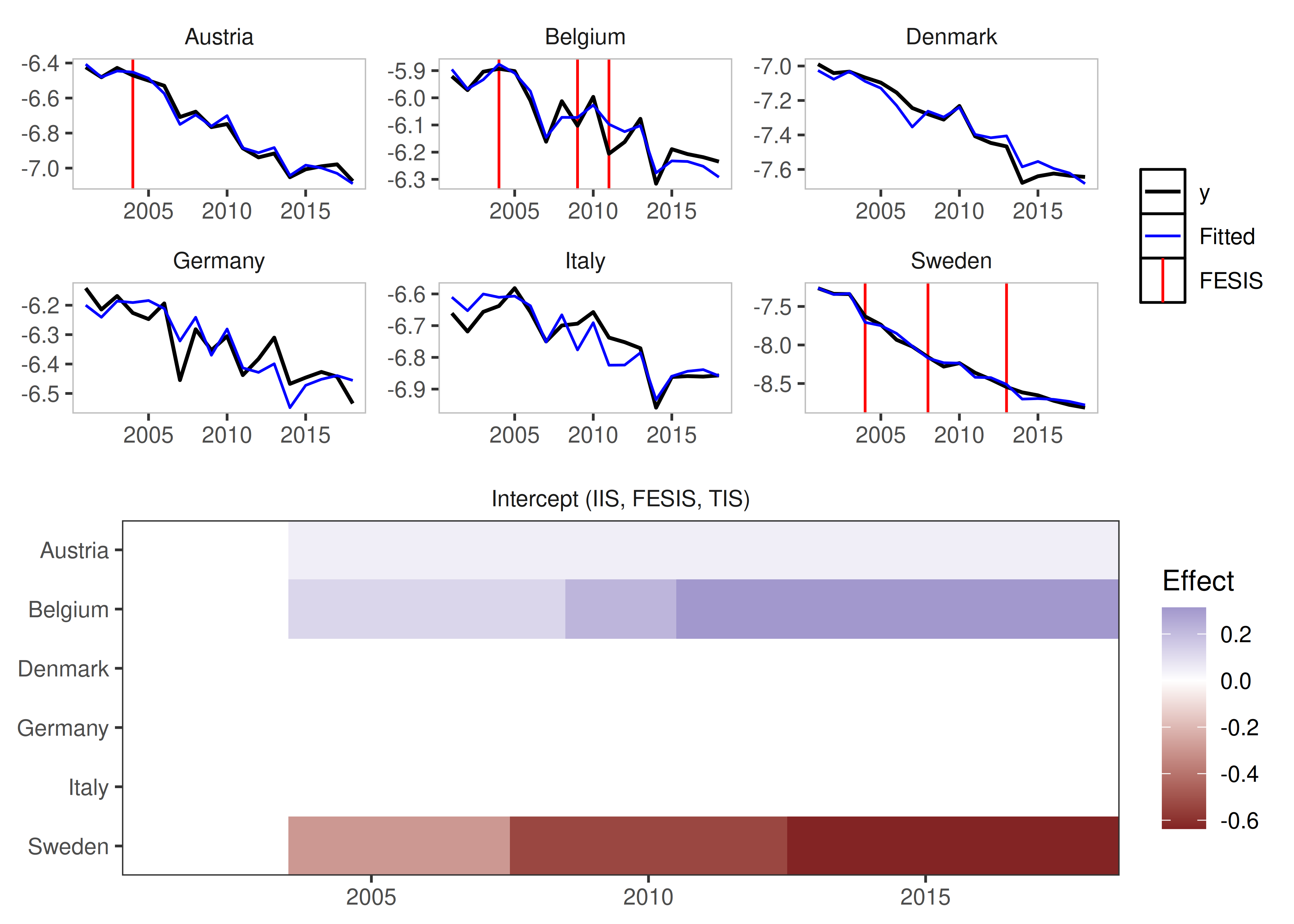

Using the traditional method

is_gets <- isatpanel(y = EUCO2residential$lagg.directem_pc,
                     mxreg = EUCO2residential$lgdp,
                     time = EUCO2residential$year,
                     id = EUCO2residential$country,

                     effect = "twoways",

                     fesis = TRUE)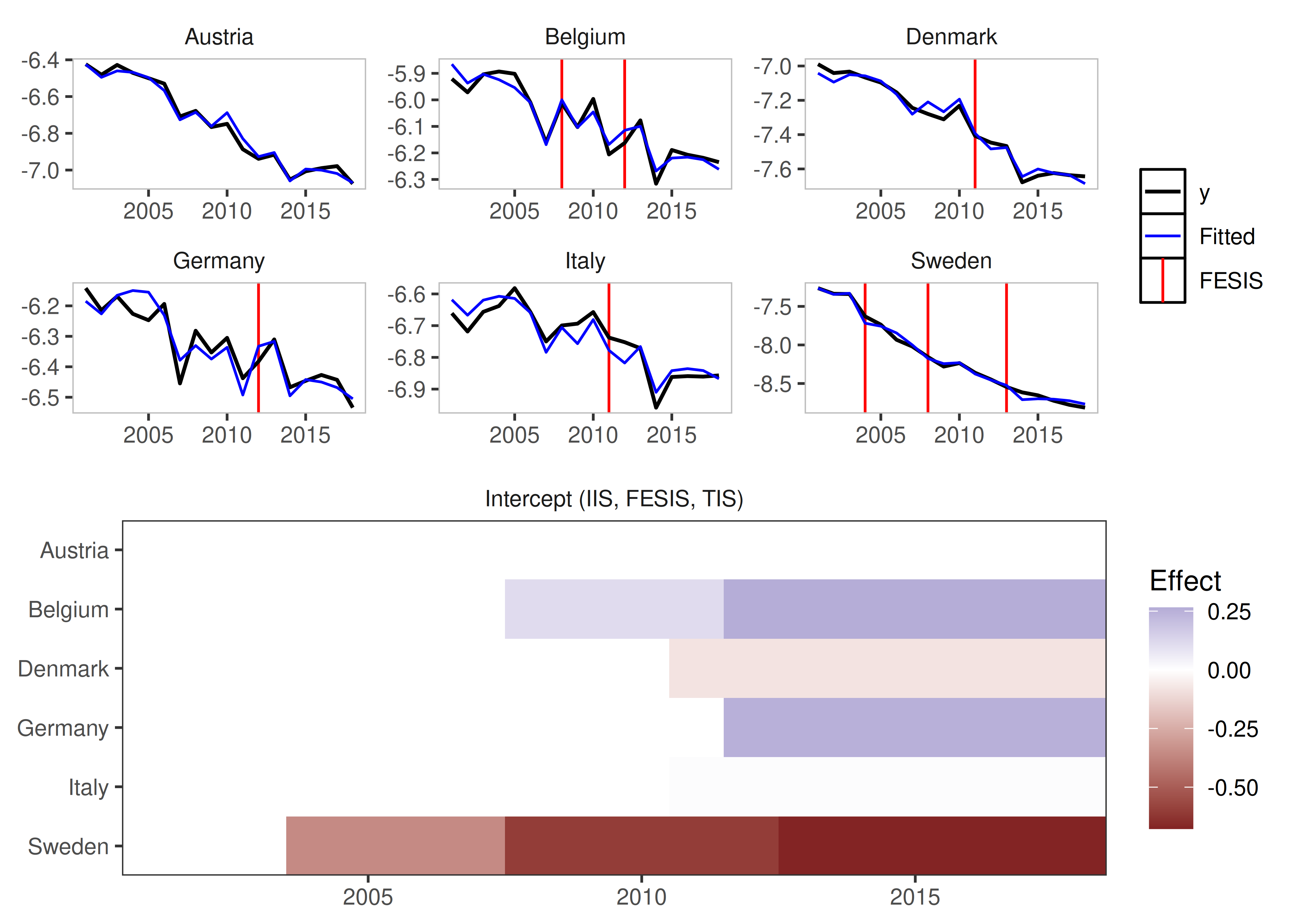

From here onwards, I will use the lm notation.

Plotting

We can plot these simply using the default plotting methods (rely on the ggplot2 package):

plot(is_lm)

plot_grid(is_lm)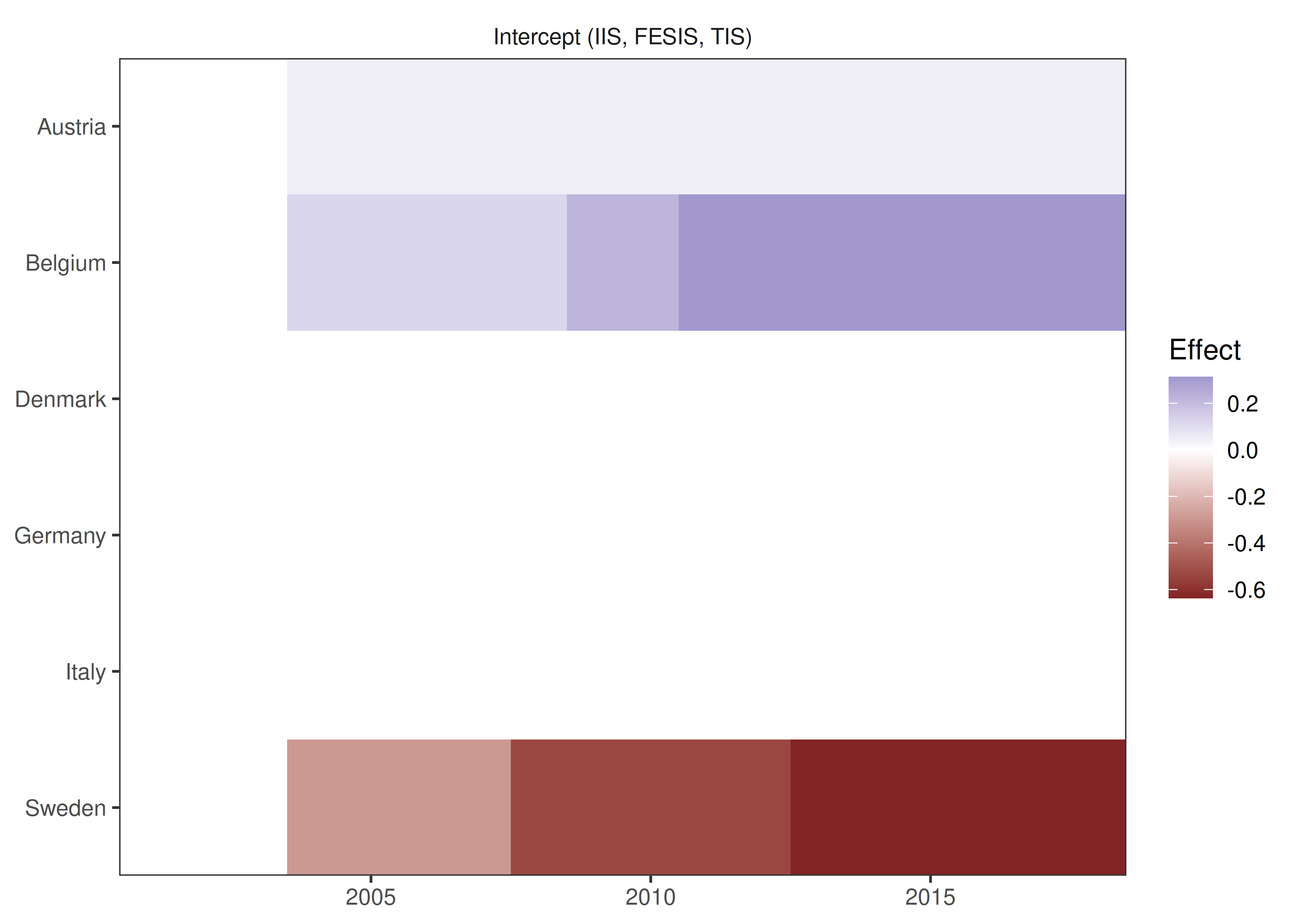

plot_counterfactual(is_lm)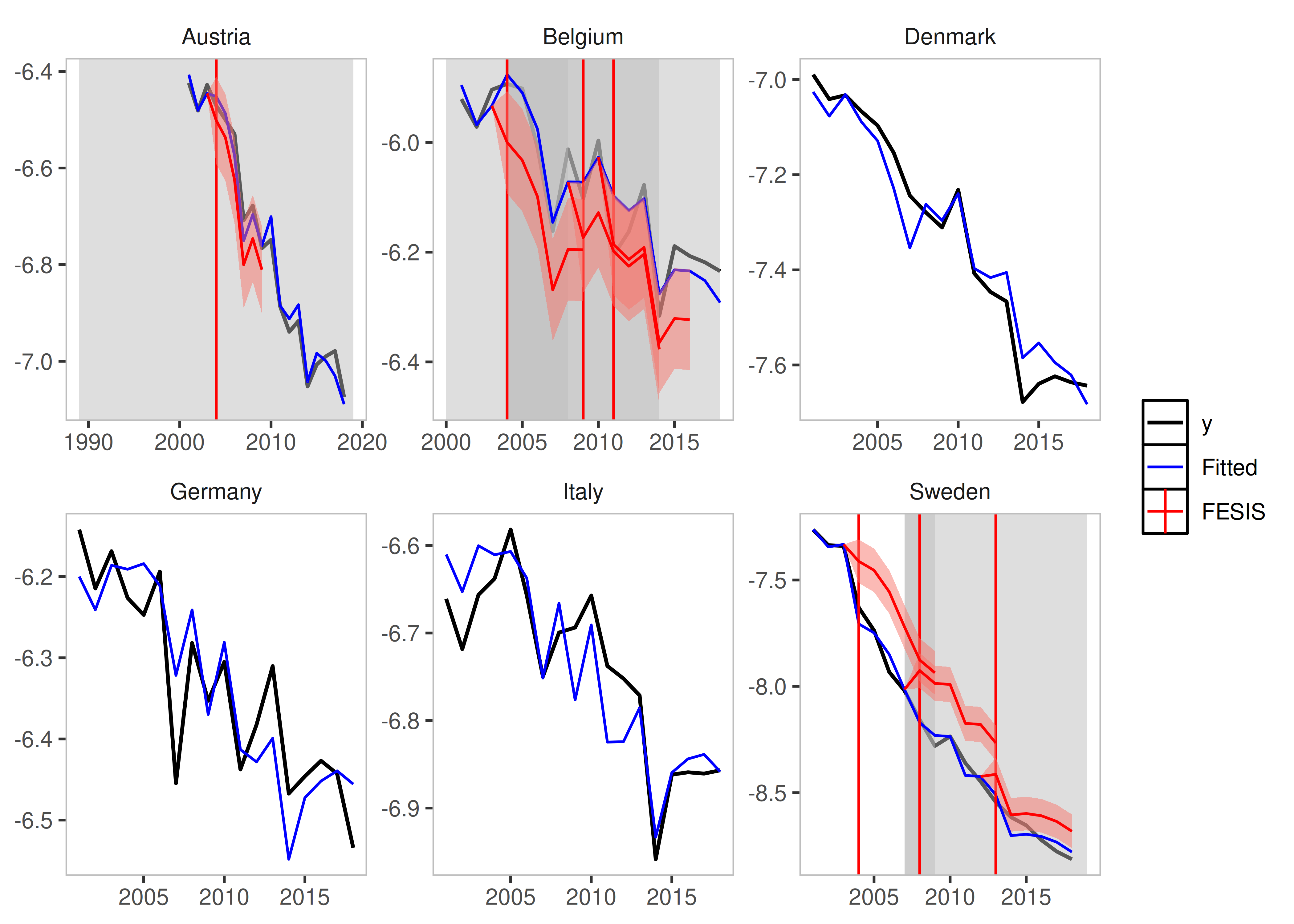

Saturation Methods

Impulse Indicator Saturation

This argument works just as in the gets package. The method simply adds a 0 and 1 dummy for each observation.

Simply set iis = TRUE.

iis_example <- isatpanel(data = EUCO2residential,
                         formula = lagg.directem_pc ~ lgdp + I(lgdp^2) + pop,
                         index = c("country","year"),

                         effect = "twoways",

                         iis = TRUE,
                         fesis = TRUE)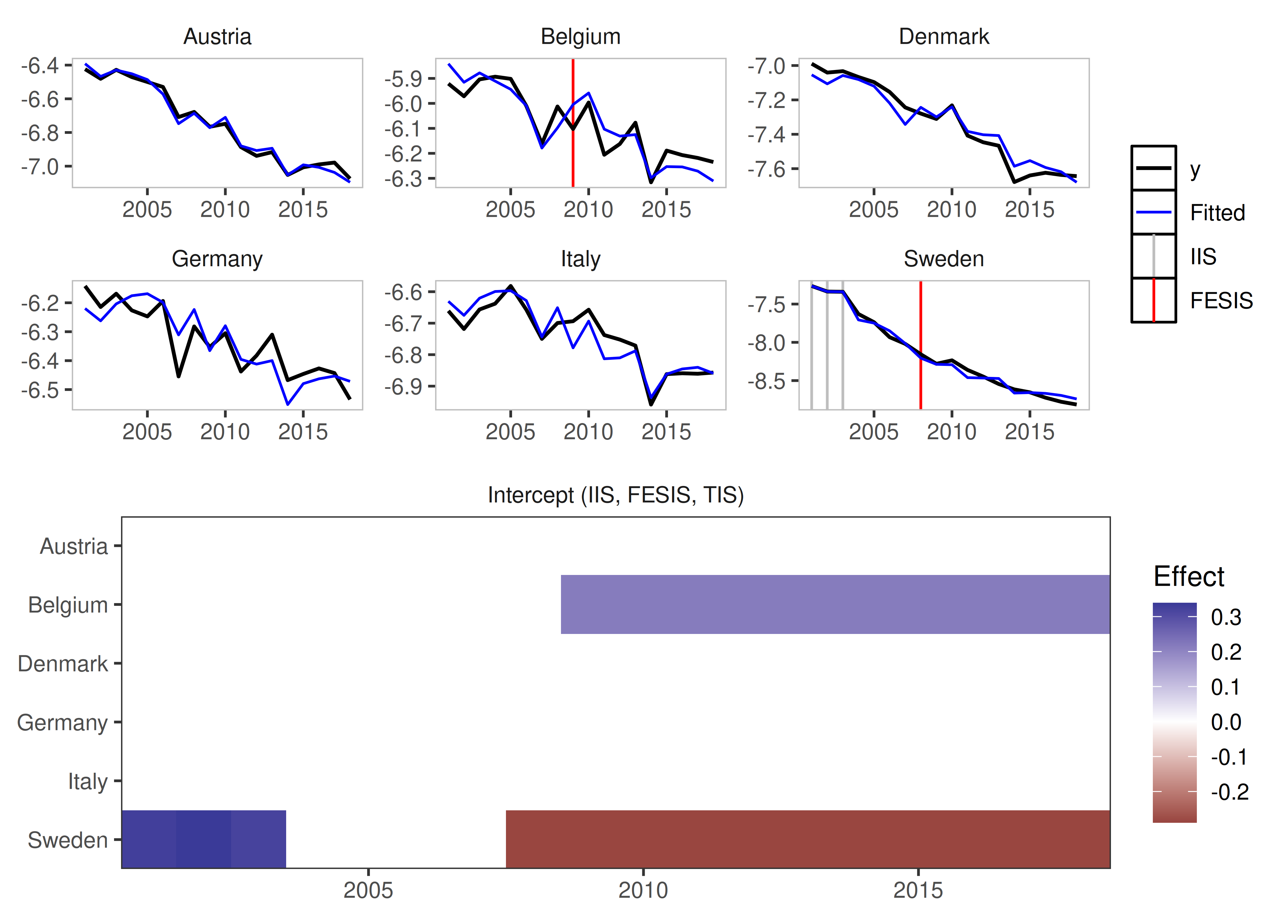

plot(iis_example)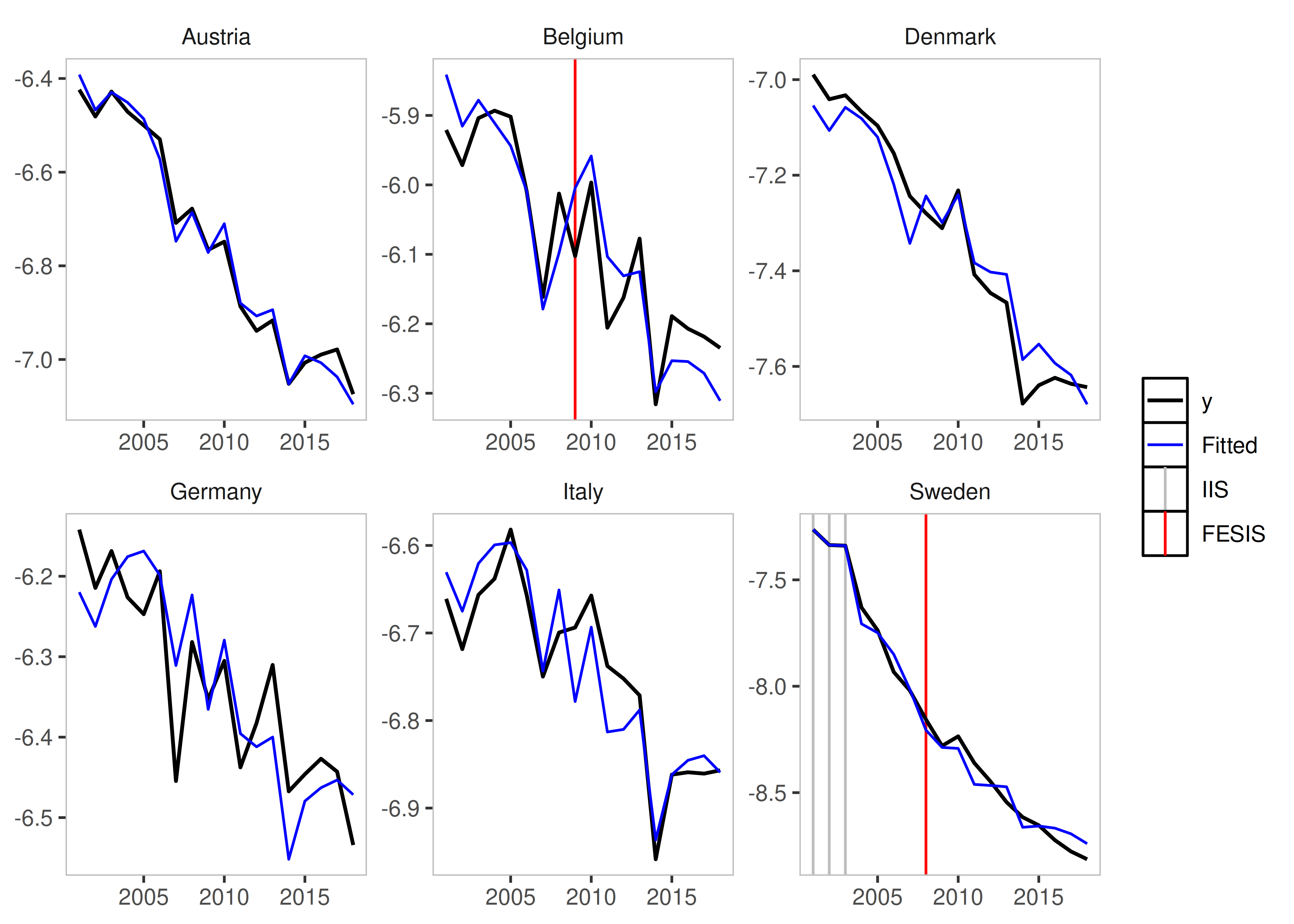

Step Indicator Saturation

Traditional Step Indicator Saturation does not make sense in a panel setting. Therefore, the gets function of sis is disabled.

Joint Step Indicator Saturation

It is possible, however, to consider Step Indicator Saturation with common breaks across individuals. Such indicators would be collinear, if effects = c("twoways") or effects = c("time") i.e. if Time Fixed Effects are included.

If, however, effect = "individual" then we can use jsis = TRUE to select over all individual time fixed effects.

jsis_example <- isatpanel(data = EUCO2residential,
                          formula = lagg.directem_pc ~ lgdp + I(lgdp^2) + pop,
                          index = c("country","year"),

                          effect = "individual",

                          jsis = TRUE)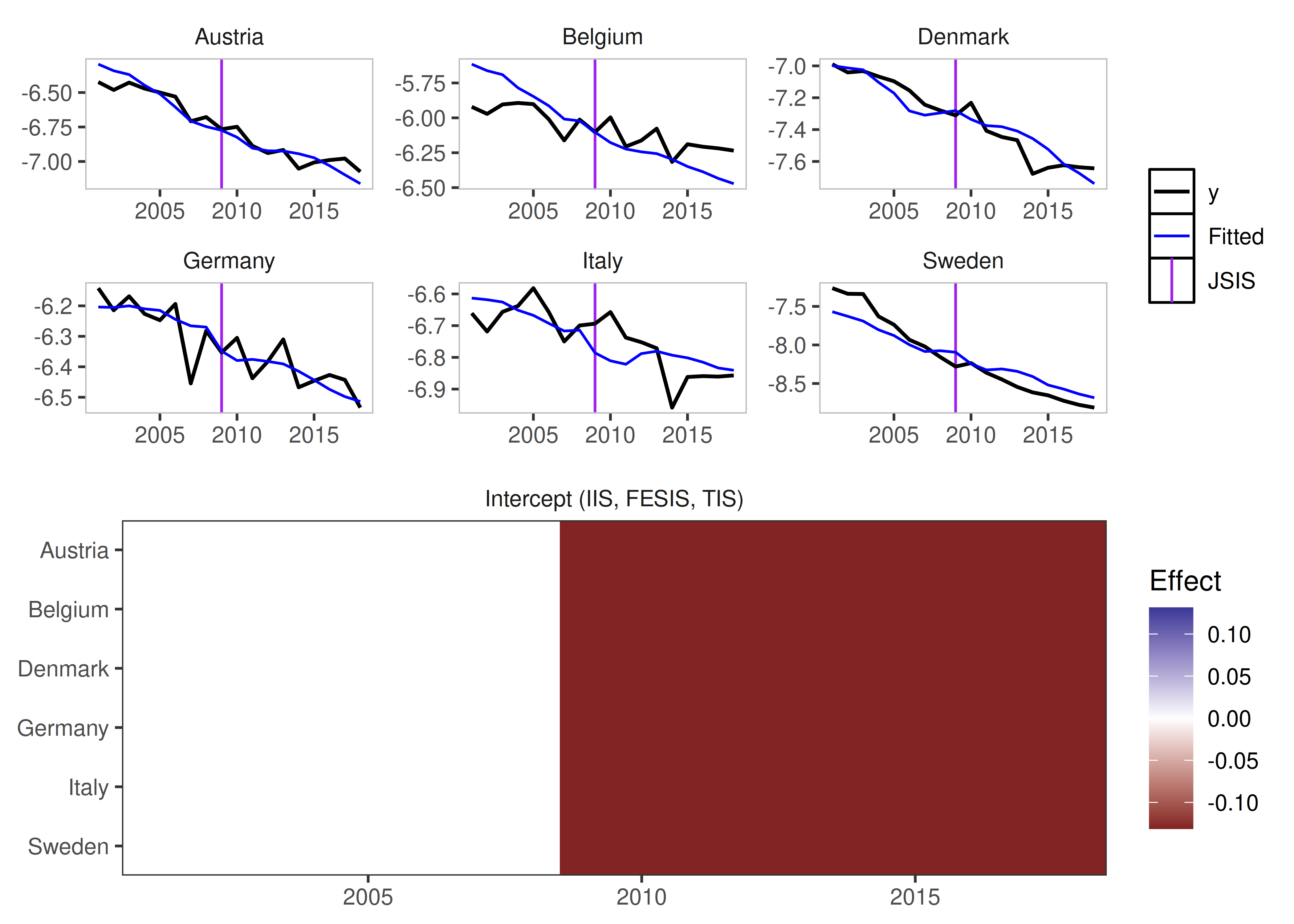

Coefficient Step Indicator Saturation

Note: This method has only been tested using the lm implementation (using data, formula, and index).

This method allows detection of coefficient breaks that are common across all groups. It is the interaction between jsis and the relevant coefficient.

To illustrate this, as well as the advantages of using the lm approach, we include a non-linear term of the lgdp variable using I(lgdp^2):

csis_example <- isatpanel(data = EUCO2residential,
                          formula = lagg.directem_pc ~ lgdp + I(lgdp^2) + pop,
                          index = c("country","year"),

                          effect = "twoways",
                          t.pval = 0.05,

                          csis = TRUE)

By default, all coefficients will be interacted and added to the indicator list - but his can be controlled using the csis_var, which takes a character vector of column names i.e. csis_var = "lgdp".

csis_example2 <- isatpanel(data = EUCO2residential,
                           formula = lagg.directem_pc ~ lgdp + I(lgdp^2) + pop,
                           index = c("country","year"),

                           effect = "twoways",

                           csis = TRUE,
                           csis_var = "lgdp")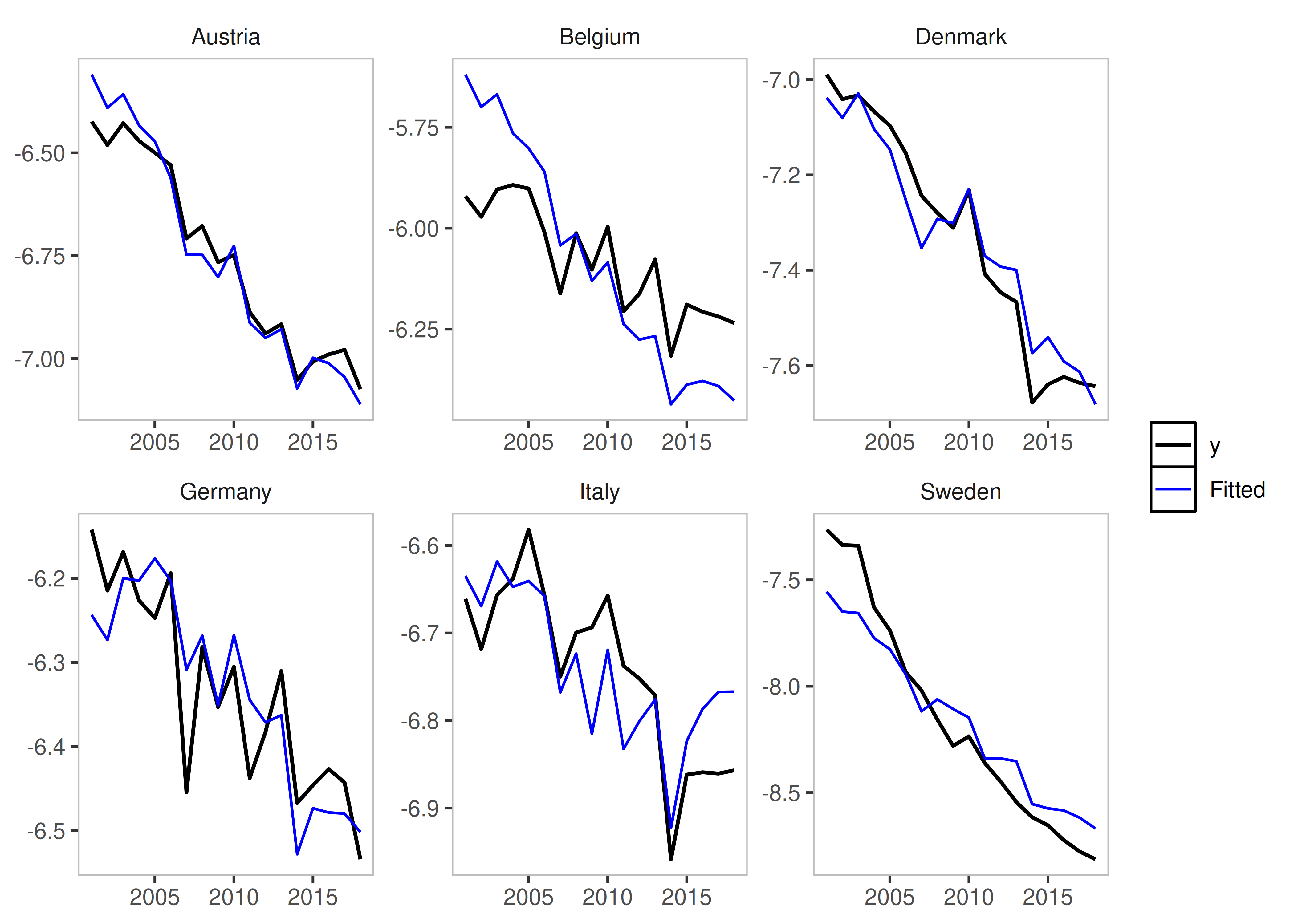

Fixed Effect Step Indicator Saturation

This is equivalent to supplying a constant to the mxbreak argument in the old method. This essentially breaks the group-specific intercept i.e. the individual fixed effect.

fesis_example <- isatpanel(data = EUCO2residential,
                           formula = lagg.directem_pc ~ lgdp + I(lgdp^2) + pop,
                           index = c("country","year"),

                           effect = "twoways",

                           fesis = TRUE)

plot(fesis_example)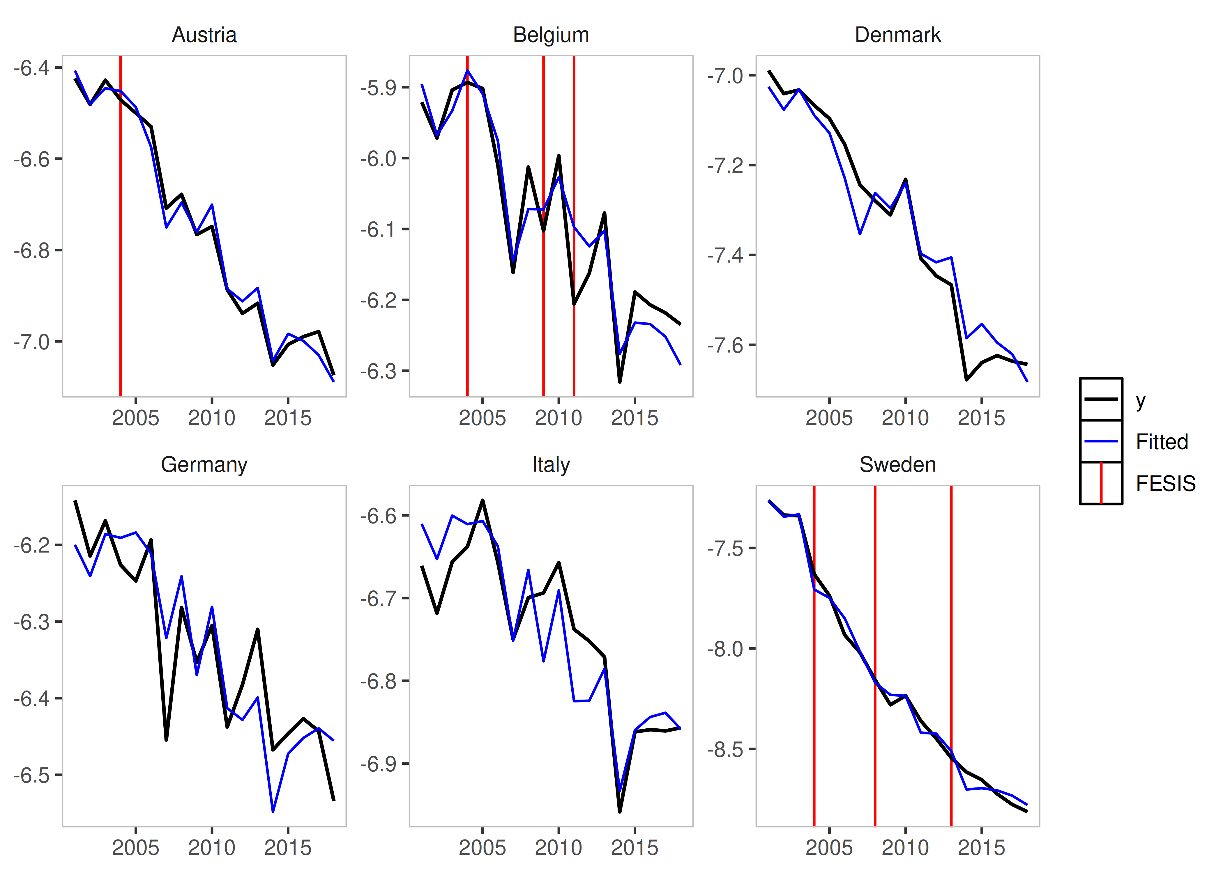

Similar to the csis_var idea, we can specify the fesis method for a subset of individuals as well using the fesis_id variable, which takes a character vector of individuals. In this case we can use e.g. fesis_id = c("Austria","Denmark").

fesis_example2 <- isatpanel(data = EUCO2residential,
                           formula = lagg.directem_pc ~ lgdp + I(lgdp^2) + pop,
                           index = c("country","year"),

                           effect = "twoways",

                           fesis = TRUE,
                           fesis_id = c("Austria","Denmark"))

plot(fesis_example2)

Post-selection robustness

The options for the robust_isatpanel are to use HAC Standard Errors, use a standard White Standard Error Correction (with the option of clustering the S.E. within groups or time):

robust_isatpanel(fesis_example, HAC = TRUE, robust = TRUE, cluster = "group")
Error in solve.default(crossprod(demX)): system is computationally singular: reciprocal condition number = 1.00556e-17

Coefficient Fixed Effect Step Indicator Saturation

This method combines the csis and the fesis approach and detects whether coefficients for individual units break over time.

This means we can also combine the subsetting in both the variable and in the individual units using cfesis_id and cfesis_var.

cfesis_example <- isatpanel(data = EUCO2residential,
                            formula = lagg.directem_pc ~ lgdp + I(lgdp^2) + pop,
                            index = c("country","year"),

                            effect = "twoways",

                            cfesis = TRUE,
                            cfesis_id = c("Belgium","Germany"),
                            cfesis_var = "lgdp",
                            t.pval = 0.001)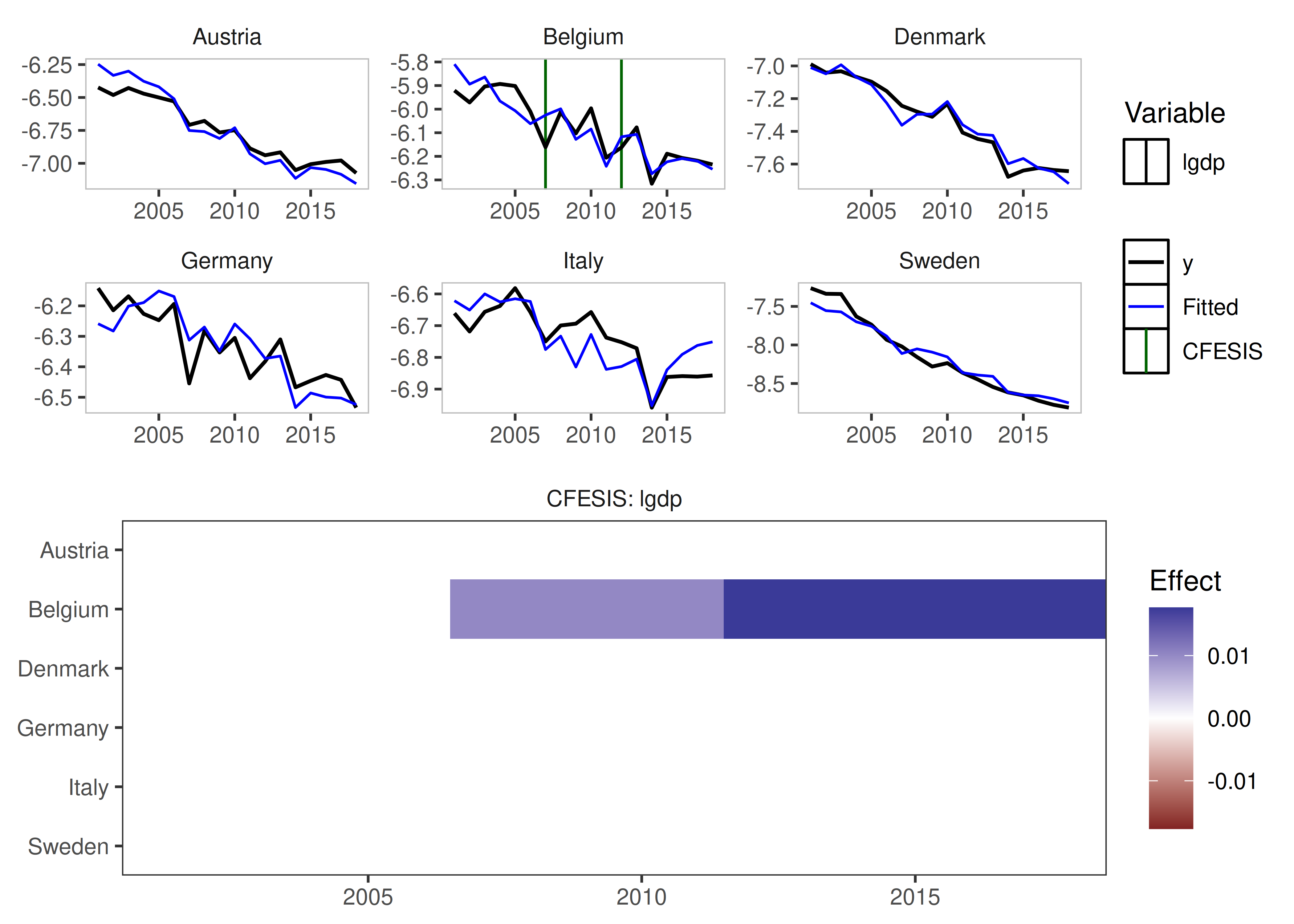

plot(cfesis_example)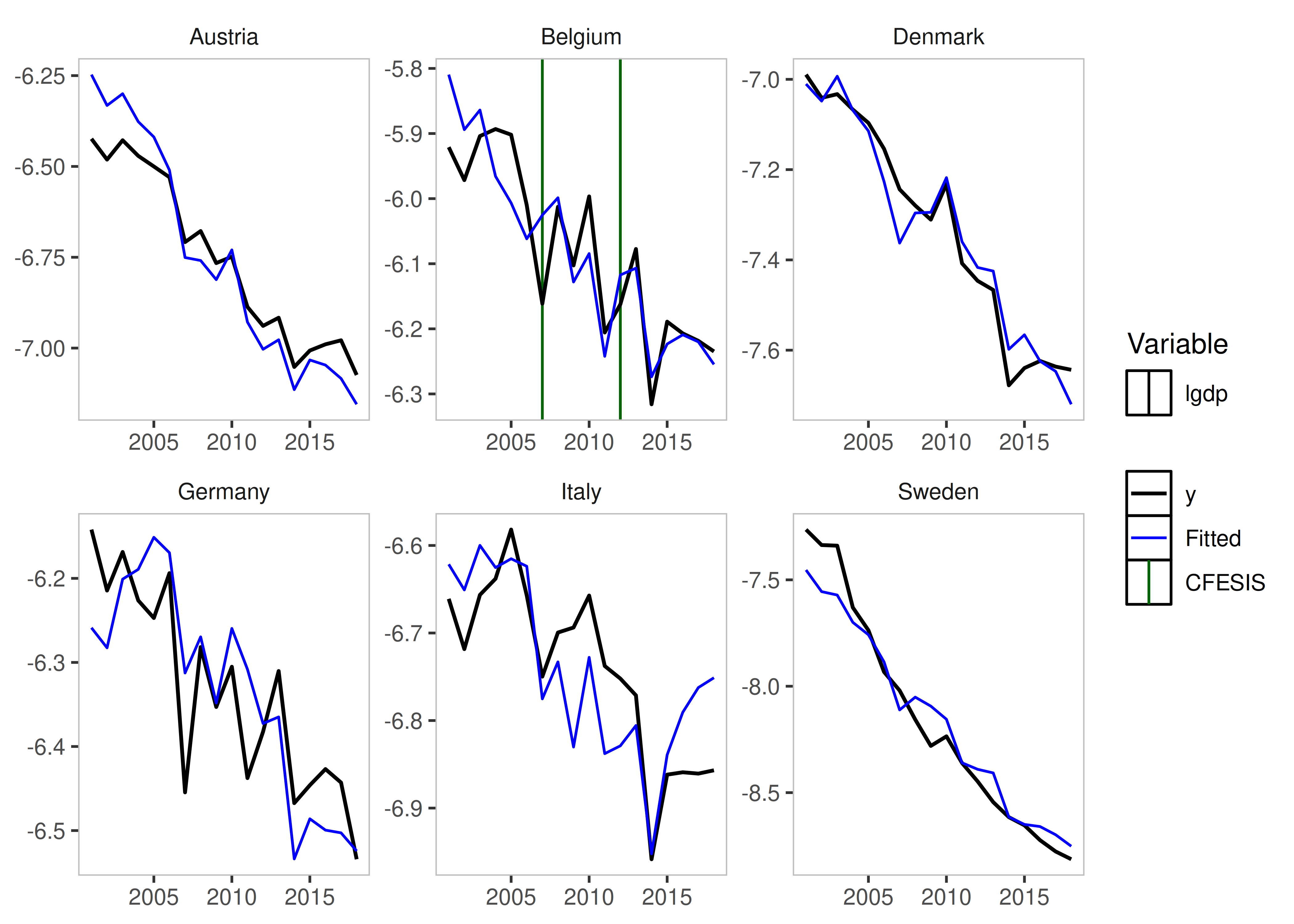

The `ar` argument

It is now possible to specify an argument to include autoregressive coefficients, using the ar argument.

fesis_ar1_example <- isatpanel(data = EUCO2residential,
                               formula = lagg.directem_pc ~ lgdp + I(lgdp^2) + pop,
                               index = c("country","year"),

                               effect = "twoways",

                               fesis = TRUE,

                               ar = 1)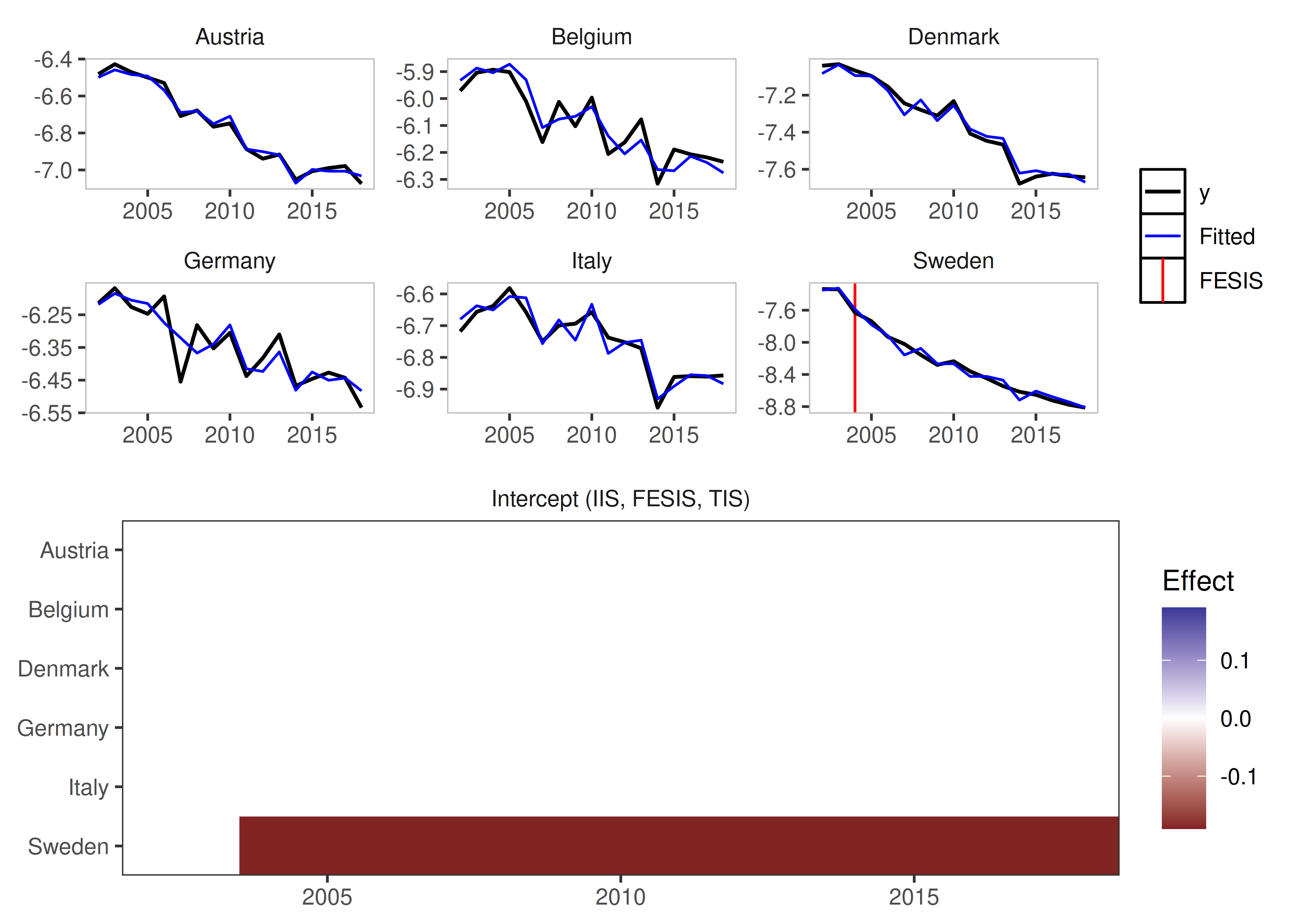

The `engine` argument

Another new argument is also the engine argument. This allows us to use an external package to estimate our models. At this stage, the fixest package can be used.

This also means that we can now use an argument to cluster Standard Errors using cluster. The following few chunks are not executed by default in the vignette.

fixest_example <- isatpanel(data = EUCO2residential,
                            formula = lagg.directem_pc ~ lgdp + I(lgdp^2) + pop,
                            index = c("country","year"),

                            effect = "twoways",

                            fesis = TRUE,

                            engine = "fixest",
                            cluster = "none")

We can verify that, using no clustering of Standard Errors at all, using the fixest package does not change our estimates:

head(fixest_example$isatpanel.result$mean.results)

Compared to the default estimator:

head(is_lm$isatpanel.result$mean.results)

However, changing the cluster specification of course does. The Standard Error correction with it’s current implementation is not valid, so allows for many more indicators than true - clustering is therefore currently not recommended.

fixest_example_cluster <- isatpanel(data = EUCO2residential,
                                    formula = lagg.directem_pc ~ lgdp + I(lgdp^2) + pop,
                                    index = c("country","year"),

                                    effect = "twoways",

                                    fesis = TRUE,

                                    engine = "fixest",
                                    cluster = "individual")

plot(fixest_example_cluster)